PUBLIC clamour for emissions reduction and energy saving, combined with sometimes low levels of knowledge among large energy users, has created fertile territory for the snake-oil pedlars.
Now some energy-saving products and techniques always work: fitting a properly-sized high-efficiency electric motor, for example. Some, like condensing boilers and voltage reduction, only work in the right circumstances. Some will work only if properly commissioned and operated (automatic lighting controls are a case in point). Some products, like those based on automatic control algorithms, may be perfectly good from some vendors but not others. Certain products, however, will never save energy under any circumstances because they are bogus. The Advertising Standards Authority ruled in 2013, for instance, that Blue Carbon Ltd must not claim that their “current optimization” device saves energy, because its claims could not be substantiated. But how is the hard-pressed environmental manager, facilities manager or works engineer, who may have little grounding in the subject, going to make the judgment about something which just feels wrong?
From the advertising literature that I have seen, there are a dozen hallmarks of suspicious products, which I elaborate on below. Unfortunately, the boundaries are not clear. Apart from bad science (which can be difficult for the lay person to judge), no single factor will definitively identify a bogus offering, and some (like ease of installation, testimonials, and high percentage savings) could be perfectly genuine. But I’d suggest if a product has four or more of the following attributes, there may well be a problem:
1. Failure to adhere to the known laws of science is a sure sign, and pseudo-scientific jargon should raise suspicion. Usually spurious claims can be debunked with basic school science, but not many people will remember their physics and chemistry lessons all that clearly in later life and most will just be left with that vague feeling that the claims sound wrong. Help may be needed from a trustworthy source. The UK Government’s Energy Technology List is a properly-curated resource for example, and I offer a free on-line basic science course for managers who just want to improve their ability to identify incorrect or misleading claims.
Technical inconsistencies may give the game away. The ASA’s ruling on Blue Carbon’s advertising drew attention to contradictory assertions in relation to magnetic fields. Purveyors of magnetic fuel enhancers used to pooh-pooh each others’ claims depending on whether they used permanent magnets or oscillating fields. And the vendor may inadvertently tip you off: one stated on his web site that his invention was not a perpetual-motion machine. Why would he need to say that?
A related trick is to misuse scientific truths. For example, it is true to say that when water boils in contact with a hot surface, heat transfer is greatly impeded if, rather than having discrete steam bubbles forming, they coalesce into a film; however, it is not correct to claim that this phenomenon will occur in a normal heating boiler. The term ‘boiler’ is a misnomer because the water in contact with the heat transfer surfaces remains liquid. Were steam bubbles ever to form because of localized overheating or inadequate water flow you would get popping and clanging noises (“kettling”) caused by detached steam bubbles condensing and collapsing abruptly in the water away from the surface.
2. Implausible percentage savings claims: more than anything, it is claims for savings of 20% or more which prompt people to become suspicious and contact me for my opinion. The problem is that some established technologies do achieve that (and more), so what is really at issue is the nagging question “if this is so good, why isn’t it fitted everywhere?”. Taken on its own, this is not evidence enough, although it is sometimes possible to show from engineering calculations that a claim is unlikely to be feasible. I return to this theme later but the enemy are not all stupid and there is a new breed smart enough to make a subtler pitch. Nobody would think a claim for six percent was suspicious.
3. Extreme ease of installation: it has to be just a simple additive, bolt-on, or electrical connection for two reasons. Firstly the salesman needs to put as few obstacles in your way as possible. Secondly it needs to be cheap for him to install and easy to remove (or abandon) when a diligent customer discovers it does not work.
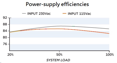
4. Being dismissive of established test methods or expertise: snake-oil merchants sometimes rubbish conventional wisdom, and when I argue with them, they point out that scientific knowledge is always advancing, that they have superior qualifications to me, that people once thought the earth was flat, etc., etc.. But however novel a product may be, its effect on losses and efficiency will be indistinguishable in kind from other products that achieve the same thing. For instance, anything which improves the efficiency of a properly-maintained heating boiler running under full load will reduce its exhaust temperature (it cannot change the residual oxygen content because that will already have been optimized). In general, if a product gives poor or no results with realistic tests, it will give poor or no results when installed.
One web site said this about people who questioned the technical basis of their claims: “they are wrong because they do not have the knowledge and technology we do”. Hmmm… A compelling argument indeed.
5. Analysis based on indirect measurements like reduced running hours: it is not safe to infer that reducing running hours reduces energy consumption. If you turn your heating off for ten minutes in every hour, for example, you will have an intermittent drop in space temperature and each time the heating system runs it will use extra fuel to restore the desired temperature. Remember in this case that heat is flowing out of the building all the time (even when the heating is off) and over the course of a day or a week, all the heat lost must be balanced by heat input, regardless of how intermittently it is supplied. In fact, to maintain the same minimum inside temperature with intermittent heat input, you would use more fuel by having to maintain a higher average.
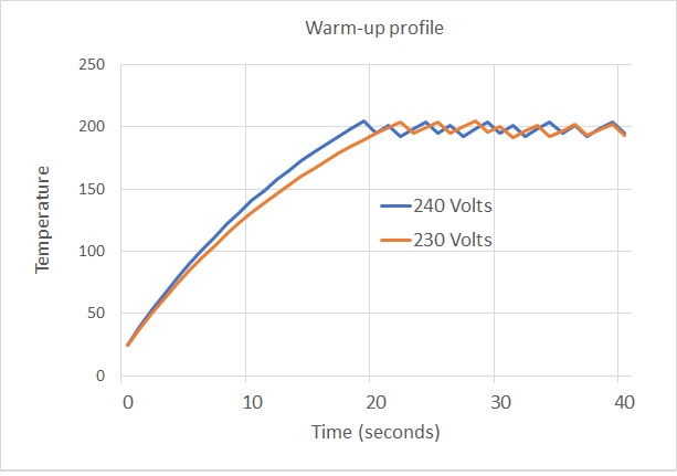
Similar considerations apply to voltage reduction, in that any reduction in current, while proving a reduction in instantaneous power, does not take running hours into account. A thermostatically-controlled electric heater in particular will run for longer in order to deliver the required quantity of heat, negating any apparent savings inferred from a spot check.
One boiler additive was promoted as having been laboratory-tested in Austria using a method based upon the time taken to boil a shallow dish of water. Really? One has to wonder why. Be skeptical of any proposal which seems to dodge direct and rigorous option of measuring actual performance before and after installation.
6. Secret ingredients or principles of operation: claims based on secrets are by their nature hard to assess in principle, so secrecy is the perfect cloak for trickery. However, if you are looking for a way to deter a persistent salesman, you can use secrecy against them. Just fall back on a health-and-safety argument. Ask for toxicity and materials-compatibility tests on any chemical constituents. And if somebody tries to sell you a magnetic device so powerful that it can affect oil or gas, ask for information about its effects on human tissue and body fluids.
7. Reliance on being patented as proof of effectiveness: have a look and see where the product is patented (if indeed it really is; sometimes vendors lie). If it is patented in the UK, at least it is probably based on accepted scientific principles. If the product is only patented in the United States or some other jurisdictions, it could be spurious because not all national patent offices require patyents to obey the laws of science. Most importantly, a patent does not imply, let alone prove, that something works; it only shows that it can be made, and how. From which it follows that if the patent refers to secret or even unspecified materials or arrangements, you can be sure you are looking at a dud because the essence of a proper patent is that it discloses enough about the invention to enable somebody with relevant skills to reproduce it.
We have recently seen a growth in references to products having been granted ‘global’ patents. There is no such thing as a global patent, so you can draw your own conclusions about anyone who says they hold one[1].
8. Heavy reliance on testimonials: I have to be careful here because good products are promoted on the basis of testimonials too. On the whole, testimonials that are purely qualitative (“the installer came at the promised time and cleaned up thoroughly afterwards”) can be believed. Quantitative ones (“we saved 30% off our gas bills”) are weak. Very few end users have the measurement and verification skills necessary to make such a claim credible. Could I just thank the hostages who smuggled out the truth in their testimonials (“the savings were unbelievable”).
Fraudsters are canny. They can harvest true testimonials from cases where there are apparent savings while ignoring the cases where there was no effect or where consumption increased. And they can blackmail their customer: who wants their boss to learn that they would not endorse a product on which they had forked out a large amount of their employer’s money? In the 1990s one case was reported to me where employees of blue-chip companies were even offered “access payments” (bribes in other words) to show prospective customers their installations.
9. Literature plastered with ISO9001 and other certification logos: sometimes it seems only the 25-yard swimming certificate has been left out. Just have a look at the certifications to see if any of them relate to efficacy.
One of the things which seemingly lends credibility is a reference to the International Performance Measurement and Verification Protocol (IPMVP). Just remember, though, that IPMVP cannot be used to validate a technology in general. It strictly covers the evaluation of a specific installation. Therefore any generic claim of savings based on IPMVP should be treated as misleading. Furthermore, under IPMVP the findings of an evaluation are valid only for the duration of the post-installation test: as soon as measurements stop, any further savings can only be presumed. They are not proven.
10. Dense academic research reports: aware of the skepticism which greets their pseudo-scientific explanations of secret (and yet patented) technologies, vendors sometimes add scientific research reports to the mix.
Of course to most prospective buyers, pages of indecipherable formulae and diagrams can do no more than create the impression of rigour and—paradoxically—increase rather than reduce their suspicions. So the reports’ authors are often (a) professors and (b) held out to be “world-leading” authorities, just to reassure you. But physics is physics and maths is maths and if such a report falls into the hands of someone independent who knows these subjects, flaws may become apparent (lines of magnetic flux do not bend abruptly; the heat transfer process in a low-temperature hot-water boiler does not include film boiling; and so on). Pointing out errors in a paper with a “world-leading” professor’s name on the cover causes indignation, online abuse and sometimes threats, but of course the vendor cannot risk going back to the professor, because the professor (even if they existed and had signed the report) will agree that some junior research assistant made those fundamental errors which had survived world-leading professorial scrutiny.
11. Name-dropping: watch out for product literature embellished with superfluous references designed to reinforce their credibility. Fair enough to say that a product has been evaluated using degree-day; but why data “from Oxford University” especially? Another favourite of mine is a product “discovered by an ex-NASA scientist”.
12. Pincer-movement sales tactics: victim energy managers can find themselves under pressure from two directions: a salesman on one hand, and a top person from their own organization who has been groomed by a director of the sales company. Often the senior contact is made socially (the “funny handshake on the golf course” approach) and it is designed to exploit the fact that senior people usually know little if anything about technical details. The energy manager is then put in the potentially difficult position of having to explain to his or her boss why the idea they are being told to follow up is stupid. This indirect bullying is a pernicious tactic because it undermines both the credibility of the energy manager and the trust between them and senior management.
Further information: to see other articles on this subject please follow this link. And generally if you are ever offered anything suspicious, feel free to ask my opinion.
————————————-
[1] There is a pilot scheme called the Global Patent Prosecution Highway but that is actually an administrative process whereby patents granted in one country will have their applications accelerated in other participating jurisdictions. The name signifies a global prosecution highway for patents, not a prosecution highway for global patents.

 Let’s be realistic: unnecessary lighting doesn’t waste much electricity. But unfortunately it is the most visible indicator of one’s commitment. It’s no good feeding children piffle about sustainability if you demonstrate a disregard for proper management of energy.