Following my retirement as an energy consultant in 2024, VESMA.COM LIMITED has ceased trading and is now dormant. I am still providing some of the company’s former services on a sole-trader basis but they are being phased out and discontinued. Specifically:
The free Meterpad service, which provides an online facility for recording and replaying manual meter readings, is no longer supported. At the time of writing it is still functioning but the plan is to terminate the service at the end of December 2026. In the event of technical failure before then, it may not be possible to reinstate it. Users are advised to (a) retrieve and archive their collected data and (b) make alternative arrangements for data collection.
Degree-day data on subscription will continue until the end of December 2026 and all active subscriptions will be extended until then. Subscribers will be notified if an alternative provider comes forward but users are advised to seek alternative sources.
Free UK degree-day data will cease to be provided in June 2026.
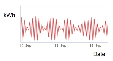
Jonathan M., a reader of my Energy Management Register bulletins, sent me an interesting query about some electricity meter readings from a closed building. Here is a picture of its half-hourly consumption over a couple of days and you can understand why he thought there must be some kind of meter error “possibly involving harmonics”:
To me the pattern was reminiscent of the ‘beating’ that you get between two sounds or electrical oscillators of similar frequency. How could that be? Figuring that one of the frequencies must be the meter-reading frequency (2 per hour) I speculated that a single load coming on and off regularly at approximately the same frequency would explain the observed waveform. Let’s put some numbers to that. Imagine a 6kW immersion heater that’s cycling on and off with no hot water being drawn. Now suppose it just happens to be on for 31 minutes and then off for 30 minutes each time. Every so often there would be a half-hour in which the heater is on for the whole time (consuming 3 kWh), followed by one in which it only registers for one-thirtieth of the interval (so 0.1 kWh). In the chart, those are the successive readings with the biggest swings. Fifteen on-off cycles later consumption would start 15 minutes into the half-hour meter interval, registering 1.5 kWh, with an equal 1.5 kWh in the following interval (roughly). This would yield no swing between successive readings. After a further fifteen on-off cycles we’d be back to the situation where 0.1 kWh is consumed in one interval and 3 kWh in the next. Overall this would give us a pattern of alternating high and low half-hourly consumptions with the magnitude of the swings varying between maxima and minima with a 15-hour periodicity, with the minim consumptions close to zero and the maxima roughly double the mean.
Amazingly (and I still cannot quite believe it) I’ve since heard that my diagnosis was correct: an immersion heater had indeed been left energised in the unoccupied building.
MAVCON24, the UK’s energy measurement and verification conference, took place in Birmingham on 23 October, 2024. As part of the proceedings I ran an exercise on how we can measure staff engagement, particularly in sustainability, the aim being to quantify where a workforce is on the spectrum from disaffected to proactive.
We need numerical indicators because we need to measure, and more importantly track, progress. We want to establish whether interventions to improve engagement work in the first place, whether they continue to work thereafter, and where we stand relative to any improvement targets.
MAVCON has traditionally been focused on the objective evaluation of energy savings, and although that has typically related to technical energy-saving measures, staff behaviour-change now features as a significant component of most corporate energy programmes. The scope is also widening to include environmental impacts. When it comes to measuring staff engagement, therefore, purely quantitative monitoring of energy performance alone is not the answer because that only looks at energy efficiency and it is too easily confounded by coincidental impacts of other measures. Hence the need for metrics indicating the degree of engagement in its own right.
It is widely recognized that awareness and engagement on energy and sustainability reflect prevailing organisational culture. A workforce that doesn’t care about anything much will behave accordingly across the board, whereas those who have willingly engaged in improvement projects related to any aspect of their working environment are more likely to take a positive attitude in other contexts. That is useful because it means that we can observe behaviours maybe only loosely related to our primary focus, and then take what we see as a proxy for overall engagement. The first time I encountered this thinking in practice was in a factory where they periodically counted the number of safety near-miss reports: any fall-off in the number implied slipping engagement levels in general.
The recommended methodology involves identifying a set of ‘index behaviours’ (like the near-miss reports for example), which can be periodically evaluated by counting or measurement, or by scoring on a subjective scale. The scores are then combined in a weighted total. High weightings would be given to important behaviours which provide a lot of data points and can be scored objectively, while low weightings are given to infrequent or less significant phenomena or that can only be evaluated subjectively.
Combining eight measured behaviours in a quarterly index
For the MAVCON exercise we divided the audience into small groups and asked each group to think of five observable behaviours related to employee engagement (not necessarily related to energy performance). We asked them to think how they would you assign a value to each, and what weighting it should have in the overall score. To give a bit of variety, the groups worked on one of three scenarios:
1. a factory making products from round steel bar that involves cutting, bending, heat treatment, degreasing and powder-coating and using hydraulic, pneumatic and electrical equipment;
2. a rural district council with: a central office housing administrative and management staff, with meeting and training rooms, customer service desks and working space for elected members; three leisure centres operated by a contractor; and significant number of staff working away from base; and
3. a wholesale food service company with ambient, chilled and frozen warehouse storage receiving bulk deliveries from suppliers and mixed loads of product then despatched daily in refrigerated lorries to customers within a radius of 60 miles.
With eleven groups to debrief there was not time to feed back every suggestion but we harvested some headlines as follows. Firstly the factory groups came up with:
• number of energy defect reports;
• scored energy checklist; and
• amount of waste
The groups thinking about the district council proposed these:
• attendance at briefings;
• training requests;
• amount of paper used;
• number of suggestions;
• level of volunteering; and
• incidence of out-of-hours running
Finally the top ideas from the group looking at the food distribution company were:
• quality of maintenance;
• vehicle telematics data (see my comments below);
• freezer alarm frequency;
• staff absences; and
• lost product
The group identifying vehicle telematics data were thinking of it in terms of fuel performance but I suggested they could think instead in terms of purely behavioral data such as harsh braking, speeding and so on. The ‘training requests’ idea is a good one, but it was rather narrowly focussed on energy training whereas it could be broadened to encompass all requests for discretionary training of any sort. The main thing the groups tended to get wrong (in my view) was to choose behaviours that would not be easy to score or measure. ‘Quality of maintenance’ might fall into this category: I would like to see this expressed as a countable quantity even if it means focussing on some specific thing like tyre pressures or poor burner tuning where a threshold can be set. Some groups also defaulted back to energy performance, which we were trying to get away from for the reasons stated earlier.
I’d like to thank the groups’ representatives for graciously accepting some robust criticism during the debriefing and hopefully my ‘grilling’ (in the words of one of them) helped everyone understand the principle of the behavioural approach to measuring staff engagement.
The behavioural approach has a number of advantages. Firstly, it avoids the pitfalls of self-reporting where you just ask people about their attitudes. Secondly, unlike staff surveys it does not rely on achieving a high participation rate, because it inherently samples the entire enterprise. Thirdly it measures outcomes rather than intentions and fourthly it isolates engagement from other energy-saving activities. Moreover, publishing the calculation method and criteria gives cues to the workforce about what is expected of them. In that respect it works very like many corporate bonus schemes and indeed it is quite likely that there would be overlap with such schemes.
In conclusion, adopting a behavioural scorecard methodology will enable your organisation, when it embarks on an employee-engagement project, to set a target for the campaign, to assess it effect, to measure continual improvement, and to detect loss of engagement which signals a need for refresher training or other booster activity.
I would like to thank Dr Hilary Wood and the team at EEVS firstly for taking MAVCON over from me so that it can continue, and secondly for the quality of the event that they put on. This was the first face-to-face MAVCON since 2018 and it was great to see so many old friends and also to meet in person a number of people who have attended my online events over the last four years.
Now that I’ve given up providing training courses and organising other events related to energy management, there could be an opportunity for another consultancy to take up the slack as a commercial venture. Happy to provide advice to anyone that’s interested.
Incidentally for anyone who is considering it I have a good web domain for sale: energy.training.
One of the frustrations of doing road-transport energy audits is the inadequacy of the data that vehicle operators record. Unless they can download consumption and distance data from the vehicle itself, they are unlikely to have much more than fuel-purchase data complemented by unusable mileage readings (the term ‘mileage’ here includes odometer readings in kilometres).
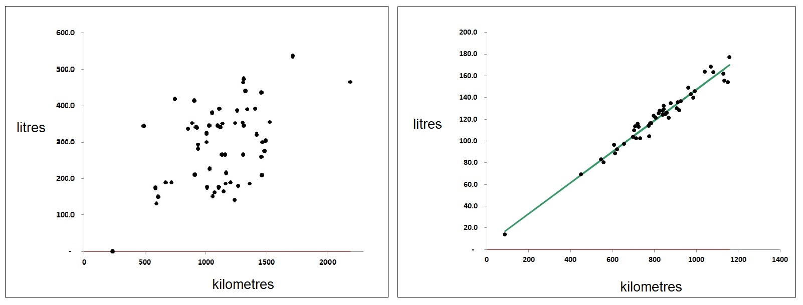
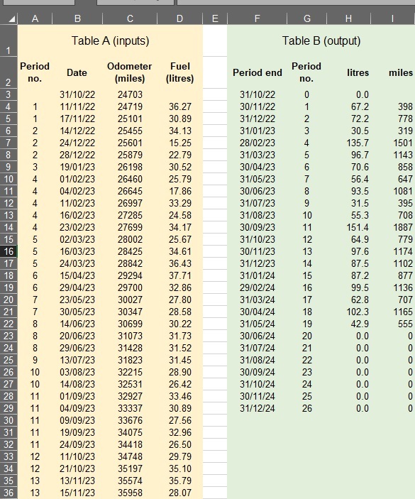
Unusable mileage figures are a major problem. For example, fuel bought on fuel cards should be accompanied by mileage records, but everyone knows that these are usually missing or incorrect. Some organisations make efforts to collect the right data but fall short: among my recent clients Company ‘S’ for example had a rigorous process for recording the daily start and finish mileages for their HGVs, along with fuel purchased during the shift, but that left huge uncertainty because a vehicle could have been refuelled at any point in a shift which could have covered hundreds of miles. And even if the mileage had been recorded at each refuelling, the driver would need to consistently brim the tank on each occasion to make the record accurate. As a result, their MPG reports were wildly erratic. In Figure 1 I compare a typical vehicle from Company S’s fleet (left) with one from Company H which collects data from its vehicles’ onboard systems:
Figure 1: weekly fuel versus distance for freight vehicles. Left: based on daily fuelling and end-of-shift mileages; right: derived from onboard consumption and distance records
Company S (on the left) can probably get a reasonable estimate of annual MPG for each vehicle but not much more. Company H, on the other hand, can detect deviations from expected fuel economy on a weekly basis and intervene promptly wherever it has deviated significantly. For sustained deviations they can also discern the nature of the change and discriminate between fixed and mileage-related excess consumption.
For vehicles where telemetry data are not available, the user needs to adopt a recording protocol that will yield accurate consumption and distance data at regular intervals. Of course this is not as straighforward as it might be for metered consumptions, because you cannot get a fuel ‘reading’ at the end of each period (week or month). The trick I have settled on is this: the data points for each period consist of (a) the sum of all fuel taken during the period and (b) the mileage between the last fill of the period and the last fill of the previous period.
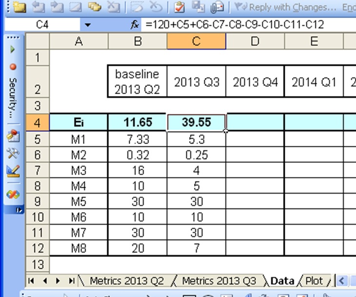
Figure 2 illustrates a spreadsheet in which this is method is used for a monthly review.
Figure 2
Note it is crucially important that drivers consistently fill their tanks to the brim. Actual refuelling data go in Table A, columns B, C and D, while the regularised monthly litres and mileage are calculated in Table B. What links the tables is a column of ‘Period numbers’. They are defined in Column G as simply the sequential row number of the table, and in column A they are calculated by looking up the Table A date in column B. Thus by way of an example the Table-A entries for 03/08/23 and 14/08/23 belong to period 10 .
Meanwhile in Table B…
the logic for calculating the incremental distance just looks up, in Table A, the finish mileages for the current and previous periods based on the period-end dates (and takes the difference); while
the litres value uses a SUMIF() function to summate all the values in Column D that have the matching period-number in Column A.
There is a copy of the example worksheet here for anyone who wants it as a starting point for their own projects. It can be made to work on a weekly cycle simply by setting the period ends in Column F at seven-day intervals.
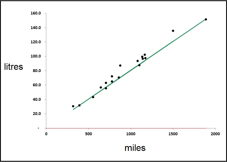
Finally Figure 3 shows analysis of monthly fuel consumption for the passenger car whose data appeared in the example above:
Figure 3: the data used in the example
Despite the random refuelling pattern, the correlation is reasonable and in fact would have been better were it not for the fact that performance was worse prior to July 2023 and from January to April 2024.
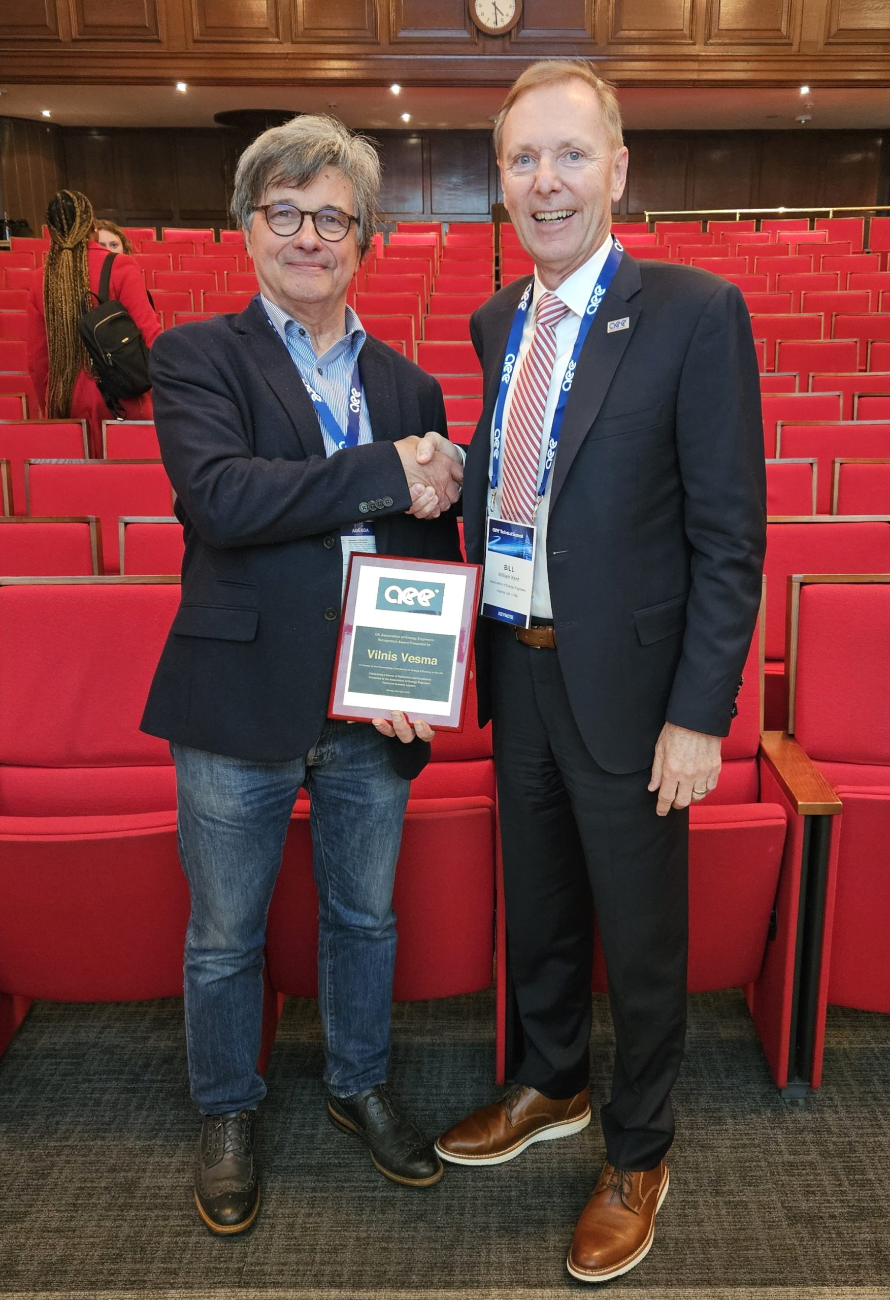
With Bill Kent of the Association of Energy Engineers after being presented with their Lifetime Achievement Award. In my acceptance speech I acknowledged just a few of the many people to whom I owe a debt of gratitude for the advice and inspiration they have given me over the years.
I’d start with Mike Horsley, a lecturer at Portsmouth Polytechnic (as it then was) and chairman of one of committees which I was responsible for servicing during my time as education officer and deputy secretary at the Institute of Energy (as it then was) in 1979-81. Mike encouraged me to render myself unemployed so that I could enrol on his 5-month full-time energy supervisors’ course, which in turn opened the door to my first job as an energy manager at Lambeth Council.
Colin Ashford was my opposite number at Hackney Borough Council and an enthusiast for personal computers, which in those days were almost unknown in the workplace. Colin invited me over to see how desktop computers could be applied to energy management, and convinced me to get one at Lambeth (where I think for a while I may have been the only person using one).
From there I moved across to Gloucestershire County Council to work with Mike Simpson, a highly experienced and competent energy manager who helped me enormously in developing my craft, and John Willoughby, our colleague who was energy manager for the local technical college campuses. John was not only an expert in energy saving in buildings (and incidentally the founding editor of Energy in Buildings magazine) but also a former lecturer who got me interested in training. It was John’s example that led to my use of models and physical aids on training courses.
While I was at Gloucestershire I had a phone call from Andrew Buckley, in more recent times director of the Major Energy Users’ Council but in those days the owner of a publishing and training business specialising in energy subjects. I’d originally encountered Andrew in my Institute of Energy days when his company had published the Directory of Qualified Energy Consultants which I had developed as an in-house reference document. Now, however, he became animated when I said I was applying desktop computers to energy management. He asked if I could do a book on the subject (which I did) and run some training courses for him… Which I did, after resigning from my job and going to my bank for a loan (£15,000 in today’s money) to buy ten computers.
Andrew had meanwhile introduced me to his colleague Dr Peter Harris who was presenting training courses on energy monitoring and targeting. It was Peter who introduced me to degree-days and cusum analysis, which completely transformed the way I went about analysing and managing energy, and became the foundation of what I subsequently did as a self-employed energy consultant. Combining the analysis techniques with the newly-emerging personal computer got me into selling energy monitoring and targeting software and providing expert advice in that domain.
For a while in the mid-1990s my brother-in-law Joe O’Keefe worked with me as a (somewhat older than average) intern because he wanted a radical change of career path. Not having much to employ him on, I gave him free rein to tinker with computers and it’s thanks to Joe that the vesma.com website appeared in 1996… The perfect gift for an ardent self-publicist like me.
Sadly some mis-steps ensued and just short of my tenth anniversary as a self-employed consultant I came close to going bust. Luckily I was rescued by Roger Hawes who was running the energy team at Torpy and Partners in Bristol and took me on when I asked for a job, something I will always be grateful for. Likewise John Mulholland who persuaded NIFES to take me on after Torpy’s became part of the Enron empire (I bailed out because I thought Enron’s European business was doomed to fail; I did not suspect the true scale of the looming disaster). John ran NIFES’s training division and was another person who helped me hone my training skills. He looked after his team exceptionally well and I remember he always had my back with the directors when I overstepped the mark.
In due course, and prompted by the financial crash of 2008/9, I left John’s team to strike out on my own once more; and while looking for collaborators and associates I renewed my acquaintance with Andrew West, who lives a few miles away and had helped me with monitoring and targeting projects in the 1990s. In the intervening years Andy had changed his career path radically and become a book-keeper. To cut a long story short he agreed to come on board and take care of not just book-keeping but other administrative tasks. It’s fair to say the business was never more successful than when Andy was there to deal with back-office distractions.
The provision of free degree-day statistics has been a cornerstone of my marketing for 35 years so it would be churlish not to acknowledge the help I got from The Thatcher Government in 1991 when they discontinued the supply of official degree-day data. It created a vacuum that I was able to fill with prominent monthly exposure in the print media, and ultimately even became a source of revenue when they were shamed into reinstating it and found that they weren’t allowed to accept a single tender from the Met.Office. But that’s a different story.
The full list of those who’ve helped me along the way would be long and in some cases complicated to explain. So with apologies to those that I haven’t mentioned I would just like to thank my loyal clients over the years and all the bulletin readers who sent in the awkward technical questions on which subsequent issues were based.
A straw poll of assessors who are in my LinkedIn ESOS group showed that 17 out of 19 have seen an upturn in requests for work, but 14 said they were turning those requests down.
Under the terms of the Energy Savings Opportunity Scheme (ESOS) Regulations 2014, the UK’s large private-sector undertakings have to assess their major energy uses every four years to identify cost-effective energy-saving opportunities. They are then supposed to notify compliance through the government-appointed scheme administrator, the Environment Agency (EA), before 5 December 2023. Compliance must be assessed and ‘signed off’ by a registered lead assessor.
We’re currently in the third compliance period, reporting on energy audits—which may have been carried out at any time since December 2019—related to the participants’ assets and corporate structures as they stood on 31 December 2022.
The issues
A number of participants have completed their assessments, and had them signed off, but the EA has failed to open a notification system[1] because it plans to change some of the requirements. Some of the proposed amendments to ESOS are potentially onerous, notably the extension—from 90% to 95%–of the proportion of energy use that a participant must audit. For many, that will mean suddenly having to add marginal minor energy uses where the cost of assessment is disproportionate to any possible gains. Vehicle fuel is the classic example.
The EA has been issuing guidance to participants (most recently on 24 May 2023) which assumes that the ESOS regulations will indeed change before 5 December. Although likely, it is not certain that they will change[2], which could potentially lead to participants undertaking needless extra work. This incidentally puts participants’ energy auditors and lead assessors in a difficult contractual and commercial position. Strictly speaking the EA has no legal basis for the guidance it is currently issuing because it cannot guarantee that the regulations will change nor, if they do change, that they will be applicable to participants certified as compliant before the new regulations take effect.
As a separate issue, part of the guidance issued by the EA is a template listing information that participants will need to supply during the notification process once it becomes available. A substantial part of the information relates to matters such as the savings achieved since previous ESOS cycles, and assorted (in some cases dubious) performance metrics. This amounts to market research or impact assessment and responses to these questions ought to be voluntary since they are not at present stipulated as requirements of ESOS and there appears to be no provision for them to become requirements in any new regulations[3]. If treated as mandatory, they will further add to compliance costs.
Suggested actions
The prudent approach is to assume that Parliament will approve new ESOS regulations before 5 December and EA will force the issue, making them in effect retroactive and incidentally making the market-research questions mandatory part of the notification process. Whatever happens it is almost certain that new ESOS requirements will be in effect for the next compliance period, so the effort of setting up the necessary record-keeping and reporting now will not be entirely wasted.
However, to minimise the impact during the current ‘phase’ of ESOS I would suggest:
Lobby against any revised regulations taking effect before 5 December 2023;
If they do take effect, lobby for them not to apply to participants certified as having complied before the date that the new regulations become law;
Lobby for the exclusion from the Notification System of questions related to market research or impact assessment.
Footnotes
[1] ESOS Regulation 8(1) obliges the Scheme Administrator to establish a Notification System but Regulation 8(2) allows it to make it available to participants only when they decide it is ‘reasonable’.
[2] The Secretary of State cannot at the moment even lay new ESOS regulations before Parliament; he lost the power when the European Communities Act 1972 was repealed. The Government is relying on the successful passage through Parliament of the Energy Bill (currently with the Public Bills Committee) to restore those powers and enable new regulations to be laid before Parliament and voted into law.
[3] The writer was unable to identify any specific provision in the relevant part (Part 10) of the Energy Bill
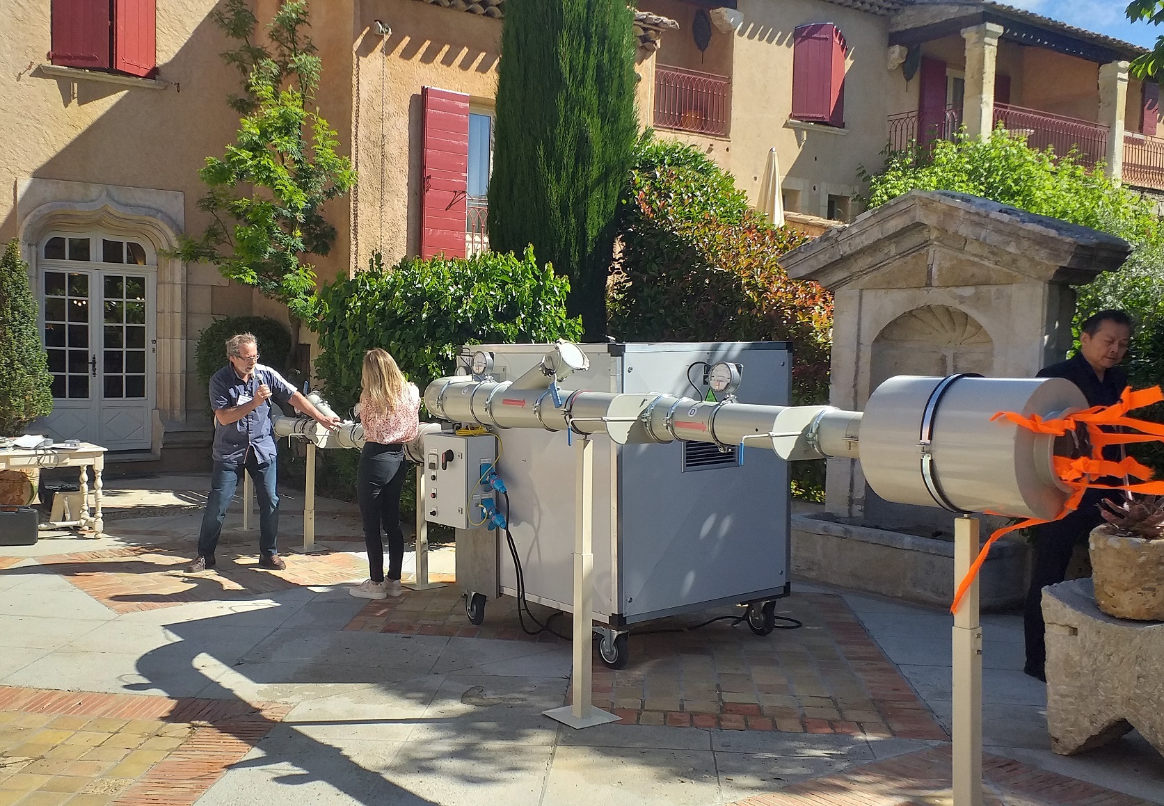
Here’s an aspect of energy saving in motor-driven systems that had never occurred to me until I went on a training course about industrial dust extraction systems. Our instructor, Christoph Ritter of Osprey Corporation (pictured on the training rig), guaranteed his audience that if he went to their factories he would find that some of their vacuum fans would be running backwards This may sound crazy, but it can and does happen. It only needs two of the motor power connections to be swapped accidentally. Centrifugal fans do still work in reverse but their efficiency becomes diabolical. If they have straight radial blades the fan-wheel itself is no less efficient but the air leaving the volute has to turn through 180 degrees, with the consequent loss of head. If the fan has backward-curved blades (normally more efficient) these are forward-curved when reversed, introducing even more loss.
The problem tends to be masked in direct-coupled fans with variable-frequency drives. One reason is that you cannot easily see the direction of rotation when there are no belts to observe; the other is that the drive system will compensate by speeding up the fan (if it can) drawing much more power to deliver the required air flow. On Christoph’s course he uses a rig to demonstrate this and a fan current of 5 amps had to go up to 22 amps to deliver the same flow when the fan motor was running backwards.