When considering the consumption of fuel for space heating, the degree-day base temperature is the outside air temperature above which heating is not required, and the presumption is that when the outside air is below the base temperature, heat flow from the building will be proportional to the deficit in degrees. Similar considerations apply to cooling load, but for simplicity this article deals only with heating.
In UK practice, free published degree-day data have traditionally been calculated against a default base temperature of 15.5°C (60°F). However, this is unlikely to be truly reflective of modern buildings and the ready availability of degree-day data to alternative base temperatures makes it possible to be more accurate. But how does one identify the correct base temperature?
The first step is to understand the effect of getting the base temperature wrong. Perhaps the most common symptom is the negative intercept that can be seen in Figure 1 which compares the relationships between consumption and degree days. This is what most often alerts you to a problem:
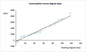
It should be evident that in Figure 1 we are trying to fit a straight line to what is actually a curved characteristic. The shape of the curve depends on whether the base temperature was too low or too high, and Figure 2 shows the same consumptions plotted against degree days computed to three different base temperatures: one too high (as Figure 1), one too low, and one just right.
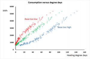
Notice in Figure 2 that the characterists are only curved near the origin. They are parallel at their right-hand ends, that is to say, in weeks when the outside air temperature never went above the base temperature. The gradients of the straight sections are all the same, including of course the case where the base temperature was appropriate. This is significant because although in real life we only have the distorted view represented by Figure 1, we now know that the gradient of its straight section is equal to the true gradient of the correct line.
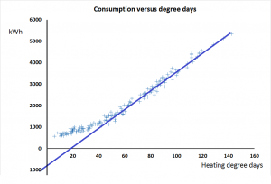
So let’s revert to our original scenario: the case where we had a single line where the base temperature was too high. Figure 3 shows that a projection of the straight segment of the line intersects the vertical axis at -1000 kWh per week, well below the true position, which from Figure 1 we can judge to be around 500 kWh per week. The gradient of the straight section, incidentally, is 45 kWh per degree day.
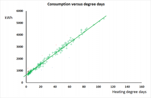
To correct the distortion we need to shift the line in Figure 3 to the left by a certain number of degree days so that it ends up looking like Figure 4 below. The change in intercept we are aiming for is 1,500 kWh (the difference between the apparent intercept of -1000, and the true intercept, 500*). We can work out how far left to move the line by dividing the required change in the intercept by the gradient: 1500/45 = 33.3 degree days. Given that the degree-day figures are calculated over a 7-day interval, the required change in base temperature is 33.3/7 = 4.8 degrees
Note that only the points in the straight section moved the whole distance to the left: in the curved sections, the further left the point originally sits, the less it moves. This can best be visualised by looking again at Figure 2.
In more general terms the base-temperature adjustment is given by (Ct-Ca)/m.t where:
Ct is the true intercept;
Ca is the apparent intercept when projecting the straight portion of the distorted characteristic;
m is the gradient of that straight portion; and
t is the observing-interval length in days
* The intercept could be judged or estimated by a variety of methods including: empirical observations like averaging the consumption in non-heating weeks; by ‘eyeball’; or by fitting a curved regression line, etc..