Clamp-on ultrasonic flow meters are tricky things to deploy and I always get a sinking feeling when somebody says they’re going to use them. In this case they were fitted to measure cooling energy as part of a measurement and verification project.  Provisional analysis in the early weeks of the project showed that all was not well: there were big apparent swings in performance, which were unrelated to what we knew was going on on the plant.

Data from the meters, which were downloaded at one-minute intervals, contained computed kWh values which I was consolidating into hourly totals. The person sending me the data was extracting the kWh figures into a spreadsheet for me but some instinct prompted me to request the raw data, which I noticed contained the flow and temperature readings as well as the kWh results. My colleague Daniel wrote a fast conversion routine which saved our friend the trouble and we discovered that there were occasional huge spikes in the one-minute kWh records which were caused by errors in the volumetric flow rates. The following crude diagram of the minute-by minute flows over several weeks shows that as well as plausible results (under 500 cubic metres per hour) there were families of high readings spaced at multiples of about 750 above that:

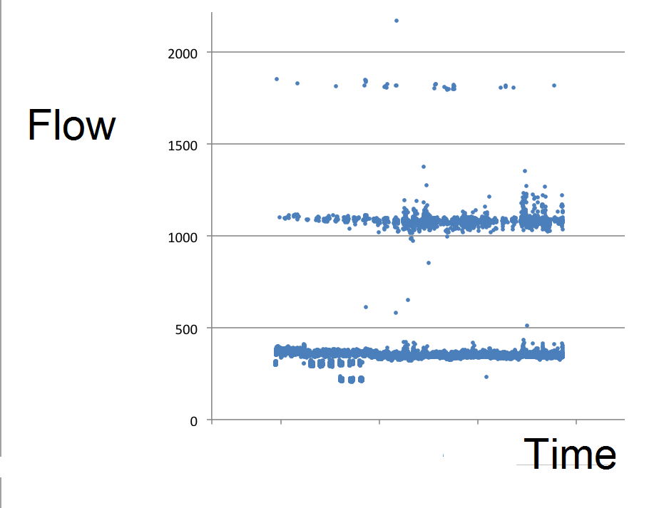
The discrepancies were sporadic, rare, and clearly delineated so Dan was able to modify his software to skip the anomalous readings and average over the gaps. We were lucky that flow rates and temperatures were relatively constant, meaning that the loss of an occasional minute per hour was not fatal. He also discovered that the heat meter was zeroing out low readings below a certain threshold, and he plugged those holes by using the flow and differential-temperature data to compute the values which the meter had declined to output.

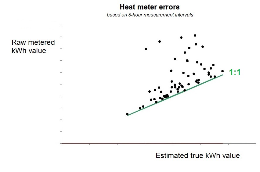
The next diagram shows the relationship between the meter’s kWh output, aggregated to eight-hourly intervals (on the vertical axis) with what we believe to be the true readings (on the horizontal axis). The straight line represents a 1:1 relationship and shows that, quite apart from the gross discrepancies, readings were anomalously high in almost every eight-hour interval.

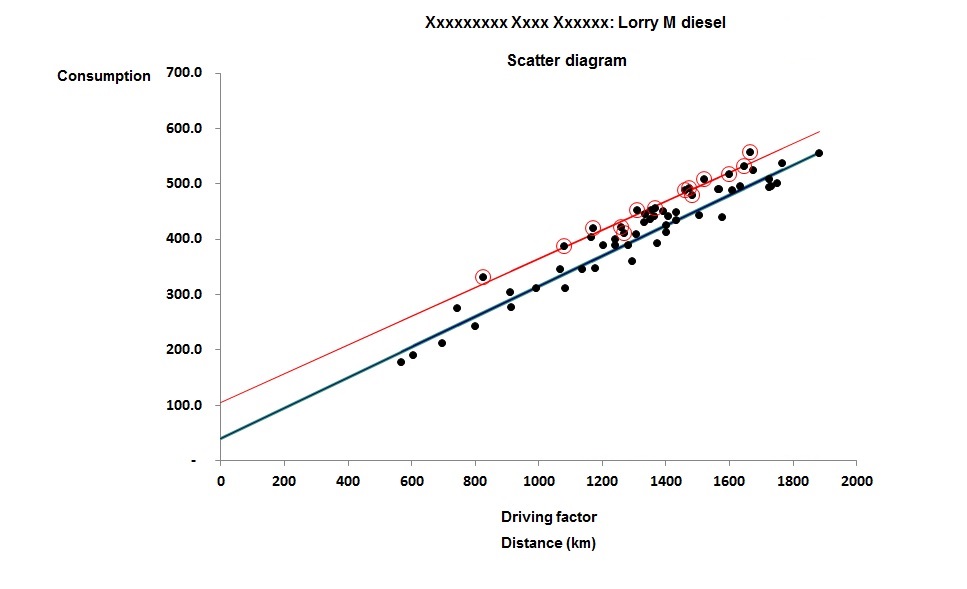
The effect on our analysis was dramatic. Instead of erratic changes in performance not synchronised with the energy-saving measure being turned on and off, we were able to see clear confirmation that it was having the required effect.

Sankey diagrams depict the flows of energy through a system or enterprise using arrows whose widths are proportional to the magnitudes of the flows.

My friend and former colleague Kevin Cardall recently challenged my newsletter readers to come up with improvements on an Excel-based Sankey Diagram generator which he had devised (illustrated right, and attached here). His work was inspired by this website. Reader David B. responded rapidly with a neat enhancement but we also had a number of alternatives suggested by other readers.

Readers’ recommendations

When the subject of Sankey diagram software came up in 2003 one of my clients recommended SDRAW.  It is a commercial product but there is a free demonstration version.

Readers Colin G., Gary C. and Chris S. mentioned a free online tool, http://sankeymatic.com/ and reader Andy drew my attention to this toolkit for those who want to do it in Excel.

ESCO in a box is a concept being developed with government support with the aim of improving takeup of energy-saving measures among small and medium enterprises.

In essence, the project is designed to enable respected local community organisations (for example) to set up as providers of energy-saving services to the SMEs in their area, by equipping them with a complete package of technical, analytical, legal and financial components.

The originators of the idea, EnergyPro Ltd, have produced an  overview of the scheme  and I interviewed their managing partner, Steven Fawkes, about it on 15 April. The recording will be available until 14 May at http://bit.ly/ESCObox  (apologies that the recording is missing the first couple of minutes).

Normally when we track vehicle performance we think in terms of miles per gallon or kilometres per litre. So in figure 1 for example we are looking at the weekly km/litre figure for a 32-tonne flatbed lorry delivering building materials:

It is just about possible to discern worsening performance towards the end of the trace. But by taking a slightly different approach we can not only confirm that there is an issue, but also learn more about its timing, nature and magnitude. We should start by plotting weekly fuel consumption against weekly distance traveled as in Figure 2. (Distance traveled is the “driving factor” in this analysis not in the sense of driving the lorry, but in the sense that variation in weekly distance traveled “drives” variation in weekly fuel use):

What we see is that there is an element of consumption (about 40 litres per week in this case) that is unrelated to distance driven. Most likely, this is fuel consumed while stationary. The straight-line relationship gives us a more precise gauge of performance because it allows us to deduce expected consumption each week quite accurately. We can thus show the deviation from expected fuel consumption as a time-history chart (Figure 3):

From this it is clear that there was a change in behaviour on or about 7 October, which manifests itself as a fairly consistent 50-litre-per week excess almost every week since (see the highlighted points).

Furthermore, we can compare the adverse and achievable behaviour on the scatter diagram (Figure 4) in which the post-change points are marked:

The red straight line is a best fit through all the post-change points, and it shows us that the apparent excess fuel consumption is not distance-related. It might be a permanent change in terrain or traffic conditions or a new pattern of deliveries with more waiting time…  Or it might be a new driver who doesn’t turn their engine off while waiting. It probably isn’t a mechanical fault, because that would tend to change the gradient of the line. But at least we know when the change occurred (which will help trace the cause), its nature (which helps eliminate some kinds of fault) and its magnitude (which helps us decide whether to bother pursuing the case).

Try getting those insights from tracking the MPG.

This method of monitoring energy performance also applies to buildings and industrial processes, and you can find training on the method at http://vesma.com/training

One of my newsletter readers, A.M., wrote from New Zealand with a series of questions about ISO50001, the management-systems standard for energy management. He has just started to get to grips with the 2018 edition. Here are his questions and my answers:

A.M.: How we distinguish between boundaries and scope? if boundary is simply the physical borders for the system (e.g. the office buildings), what is scope then? and if scope is for example “transportation” and etc., why in SEU [significant energy use] we say “Transportation” could be an SEU as a process?

V.V.: “Scope” means the range of activities covered. For example “manufacturing processes” or “heating, ventilation and air conditioning” or, as you say “transportation”. Within transportation you might have, for example, “freight” as an SEU, but equally you could declare all transport as significant. There is no paradox here.

A.M.: In the new edition, the top management shall take all the responsibilities that the representative had in the last edition. This sounds impossible to delegate all the tasks to the top management. How do we cope with this?

V.V.: If you are responsible for a task you can delegate it but still keep responsibility, i.e., it is your fault if the people you delegated it to fail to carry it out properly. Managers are accountable for the actions of subordinates.

A.M.: In section 4.3, page 8, after b) we have a statement “The organization shall not exclude an energy type within the scope and boundaries” I do not understand the idea! why we are not allowed to do so?

V.V.: The requirement seems logical to me. For one example: if you have transport as your scope and you have plug-in hybrid vehicles, it is reasonable to insist that you cannot exclude any electricity used by them. Another example: if you had an oil-fired boiler and replaced it with a wood-fired one, it would evidently be wrong to exclude the wood fuel from consideration.

A.M.: If a new opportunity would become replacing diesel boiler with wood pellet, it means we are changing the energy types which does not necessarily reduce the energy costs. Can we call it action plans?

V.V.: ISO50001 is about managing energy performance, not costs or carbon. If substituting a different fuel improves the energy performance, it will contribute to your aims and objectives, so it would make sense to classify the work as an action plan.

A.M.: I understand that for each energy type, we identify SEU(s) and for each SEU, we list the action plans. What if one action plan reduces diesel and increases electricity? Do we still keep it as an action plan for diesel?

V.V.: What matters is the overall energy performance. If the amount of electricity consumption that you add exceeds the amount of diesel energy saved, your energy performance would be worse after the project and it would therefore make no sense to include the project in an action plan within your EnMS. If the project is going to improve energy performance, you could declare it as part of an action plan.

Clare C., a regular reader of my energy-management bulletins, was perplexed when she started researching the cost advantages of LEDs as replacement for metal halide (MH) high-bay fittings. She discovered that MH lamps have luminous efficacies very similar to LEDs with both, broadly speaking, yielding about 100 lumens per watt. Certainly she wasn’t going to get the 50% saving she was after, and she asked my opinion.

There are a couple of factors that would tip the balance in favour of LEDs. Firstly, she needed to account for the fact that unlike LEDs, MH lamps need control gear which would add some parasitic load (say 20 watts on a 400-watt lamp).  Secondly, LEDs are more directional and can deliver all their output more effectively to the working space; MH lamps are omnidirectional and need reflectors which may lose some of the light output. So in terms of useful light output per circuit watt, a well-specified and correctly-installed LED fitting may have a moderate advantage.

But the big gain is in controllability. MH lamps have a warm-up time measured in minutes and a ‘restrike’ time (after turning off) which is longer still, to allow them to cool before being turned on again.  This is common to all high-intensity discharge (HID) lamps. It does not matter how long the delay is; it discourages the use of automatic control so  HID lamps are often turned on well before they are needed, and then stay on for the duration. LEDs by contrast can be turned off at will and as soon as they are needed again, they come on. This is where Clare will might get her 50% saving.

Scale build-up from hard water is often cited as a cause of energy waste in hot-water systems (I am talking here about ‘domestic hot water’ supply, not closed loops within central heating systems; I will come to those later). Actually though, contrary to claims for some water treatment devices, it is not necessarily the case that energy waste in DHW systems will be significant. Indeed with an electric immersion heater on a 24-hour service, all the supplied energy still gets into the water; there is no loss. Of course the rate at which the water temperature recovers will be reduced, and the heating element will fail prematurely, but those are service and reliability issues not energy waste.

The story is a little different on intermittent hot water storage of any kind. Here, because scaling will retard temperature recovery, users may extend preheat times and that will result in a marginal increase in standing heat loss. If the heat supply is from a primary (boiler-fed) water loop, the primary return temperature will be higher because scale impedes heat transfer, and this also will increase standing losses although in reality not to a significant extent in the grand scheme of things. If hot-water recovery times deteriorate markedly, users may of course dispense with time control altogether and in those circumstances avoidable standing heat loss might become significant if thermal insulation is poor.

Turning now to the effect on wet central heating circuits, scaling will affect efficiency. Scale within heat emitters (radiators and so on) will reduce heat transfer and result in higher circulating temperatures because the heat cannot escape from the water so readily. Meanwhile within the boiler itself, impaired transfer of heat into the (now hotter) system water will result in excessive heat going up the chimney, evidenced by elevated exhaust temperatures.

Furthermore in both heating and DHW systems, scale could interfere with the operation of control valves and either result in excessive heat output – with a corresponding excessive use of fuel – or inadequate heat output, which will cause people to interfere with the controls, deploy electric heaters, or take other actions that incur excess costs.

Preventing scale build-up

Simplifying the story somewhat, the main constituent of scale is calcium carbonate, which starts to form above about 35°C through breakdown of the more soluble calcium hydrogen carbonate that is present to varying degrees in the public water supply, with  ‘hard’ water containing higher concentrations of it. Calcium carbonate crystals of the normal ‘calcite’ form stick to surfaces and each other, and that is what constitutes limescale.

One way to deal with this is softening which (in its strict sense) involves a chemical process to turn calcium carbonate into sodium carbonate which does not precipitate as crystals but stays in solution. The process is costly in terms of chemicals; a waste product, calcium chloride, needs to be flushed away periodically; and the softened water is unsuitable for drinking and cooking because of its high sodium content.

The alternative to chemical treatment is physical conditioning. Various proprietary methods are available. Some involve electric or magnetic fields which are supposed to affect the calcite crystals in some way (for example giving them an electric charge so that they repel each other, or in some other manner inhibiting their tendency to agglomerate).

Another class of conditioner is electrolytic. Electrolytic devices release of minute quantities of zinc or iron into the water, which change the calcium carbonate to its ‘aragonite’ form which, unlike calcite don’t stick together, so they stay in suspension and do not contribute to scale formation.

For a wide-ranging introduction to energy-saving technologies look out for my one-day ‘A to Z’ courses advertised at vesma.com

With the exception of electrolytic devices, there is no scientific explanation of how or why most  of these physical conditioners work, and there are no accepted tests of efficacy. There is only anecdotal evidence, but if it works, it works.

The one method of physical condition which is definitely effective (and I can vouch for it personally) is polysilicate-polyphosphate dosing. This has a dual action. It modifies the carbonate crystals to stop them sticking to each other, and it coats the inner surfaces of pipework and appliances to inhibit scale formation.

For anybody wanting further references, this note from WRc commissioned by Southern Water is what I currently regard as the most authoritative advice on the subject of water treatment techniques.

We all know that trees are good and absorb carbon dioxide. But how good are they? Let’s work it out…

Trees absorb carbon dioxide at different rates depending upon their age, species and other factors but as a rough order of magnitude you can say the figure for a typical established tree is 10 kg per year. The carbon dioxide emissions associated with energy use are 0.2 kg per kWh for natural gas and (in the UK in 2018, including transmission losses) an average of 0.3 kg per kWh for electricity.

So 50.0 kWh of gas or about 33.3 kWh of electricity each generate the 10 kg of CO₂ that a single tree can absorb in a year. Take that figure for electricity. As a year is 8760 hours, 33.3 kWh equates to a continuous load of only 3.8W. So one entire tree compensates for one broadband router, a TV on standby, or a couple of electric toothbrushes or cordless phones (roughly).

And as for gas consumption: remember pilot lights? The little flame that burns continuously to ignite the main gas burner? If you had pilot flame with a rating of 100 watts, in the course of a year it would use 876 kWh and require no fewer than 17 trees to offset its CO₂ emissions..

Are the assumptions correct?

The first time I published this piece in the Energy Management Register bulletin my estimate of CO₂ takeup rates was challenged. Fair enough: I plucked it from stuff I had found on the Web knowing that it might be out by an order of magnitude. So let’s do a sense check.

The chemical composition of wood is 50% carbon (on a dry-matter basis) and all that carbon came from CO₂ in the air. So 1 kg of dry woody matter contains 0.5 kg of carbon, which in turn was derived from 0.5 x 44/12 = 1.833 kg CO₂ . Thus if we know the growth rate of a tree in dry mass per year, we can multiply that by 1.833 to estimate its CO₂ takeup. Fortunately a 2014 article in ‘Nature’  has the growth figures we need. Although there is wide variability in the results, for European species with trunk diameters of 10 cm the typical growth in above-ground dry mass is 1.6 kg per year, equating to a CO₂ takeup of only 2.9 kg per year (although this rises to 18 and 58 kg per year for diameters of 40 and 100 cm). So newly-planted trees (which is what we are talking about) are going to fall well short of my 10 kg/year estimate, and it will be years before they reach a size where their offsetting contribution reaches even modest levels.

I like trees – don’t get me wrong – by all means plant them for shade, wildlife habitat, fruit or aesthetic appearance. But when it comes to saving the planet I just think that given the choice between (a) planting a tree and waiting a few years, and (b) cutting my electricity demand by 3.8 watts now, I know what I would go for.

WHEN I FIRST heard the term science-based target (SBT) bandied around in the public arena I thought “oh good – they are advocating a rational approach to energy management”. I thought they were promoting the idea that I always push, which is to compare your actual energy consumption against an expected quantity calculated, on a scientific basis, from the prevailing conditions of weather, production activity, or whatever other measurable factors drive variation in consumption.

How wrong I was. Firstly, SBTs are targets for emissions, not energy consumption;  and secondly a target is defined as ‘science-based’ if, to quote the Carbon Trust, “it is in line with the level of decarbonisation required to keep the global temperature increase below 2°C compared to pre-industrial temperatures”. I have three problems with all of this.

Firstly I have a problem with climate change. I believe it is real, of course; and I am sure that human activity, fuel use in particular, is the major cause. What I don’t agree with is using it as a motivator or to define goals. It is too remote, too big, and too abstract to be relevant to the individual enterprise. And it is too contentious. To mention climate change is to invite debate: to debate is to delay.

Secondly, global targets cannot be transcribed directly into local ones. If your global target is a reduction of x% and you set x% as the target for every user, you will fail because some people will be unable or unwilling to achieve a cut of x% while those who do achieve x% will stop when they have done so. In short there will be too few over-achievers to compensate for the laggards.

Finally I object to the focus on decarbonisation. Not that decarbonisation itself is valueless; quite the opposite. It is the risk that people prioritise decarbonisation of supply, rather than reduction of demand. If you decarbonise the supply to a wasteful operation, you have denied low-carbon energy to somebody somewhere who needed it for a useful purpose. We should always put energy saving first, and that is where effective monitoring and targeting, including rational comparisons of actual and expected consumption, has an essential part to play.