WHEN you use metered fuel to heat a building (or indeed if you use the building’s electricity supply, but have no air-conditioning) it is straightforward to monitor heating performance critically because you can relate energy consumption to the weather expressed as degree days.
Things get difficult if you use electricity for both heating and cooling and everything shares a meter, as would be the case if you use reversible heat pumps (air-source or otherwise). Because the seasonal variations in demand for heating and cooling complement each other (one being high when the other is low), you may encounter cases where the sum of the two appears almost constant every week. Such was the case on this 800-m2 office building:
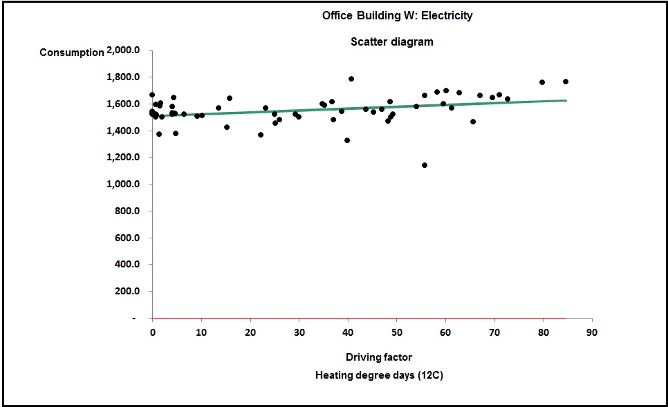
Without going into detail, this relationship implied a heating capacity of little over 1 kW, which is obvious nonsense as there was no other source of heat. The picture had to be caused by overlapping and complementary seasonal demands for heating and cooling, which is illustrated conceptually in Figure 2:
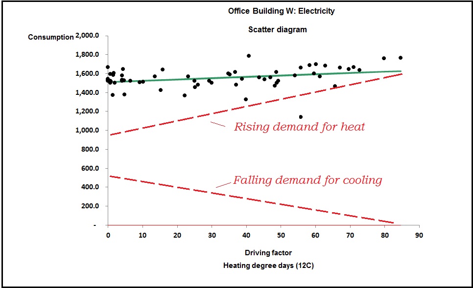
The challenge was how to discover the gradients of the hidden heating and cooling lines. The answer in this case lay in the fact that we had sufficient information to estimate the building’s heat rate, which is the net heat flow from the building in watts per unit inside-outside temperature difference (W/K). The heat rate depends on the thermal conductivity of the building envelope and the rate at which outside air enters. There is a formula for the heat rate Q:
Q = Σ(UA) + NV/3
Where U and A are the U-values and superficial areas of each building element (roof, wall, window, etc), V is the volume of the building and N is the number of air changes per hour. Figure 3 shows the spreadsheet in which Q was calculated for the building in question (an on-line tool to do this job is available at vesma.com):
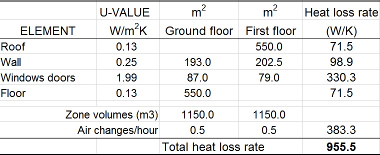
In this case the building measurements were taken from drawings, the U-values were found on the building’s Energy Performance Certificate (EPC), and the figure of 0.5 air changes per hour is just a guess.
The resulting heat rate of 955.5 W/K equates to 955.5 x 24 / 1000 = 22.9 kWh per degree day. This is heat loss from the building but it uses a heat pump and will therefore require less input electricity by a factor of, in this case, 3.77 (that being the coefficient of performance cited on its EPC). So the input energy required for heating this building is 22.9 / 3.77 = 6.1 kWh per degree day. This is the gradient of the unknown heating characteristic, the upper dotted line in Figure 2.
Need training in energy management? Have a look at vesma.com
To work out the sensitivity to cooling demand we use a little trick. We take the actual consumption history and deduct an allowance for heating load which, in each week, will be 6.1 times the number of heating degree days (remember we just worked out the building needed 6.1 kWh per degree day for heating). This non-heating electricity demand can now be analysed against cooling degree days and this was the result in this case:
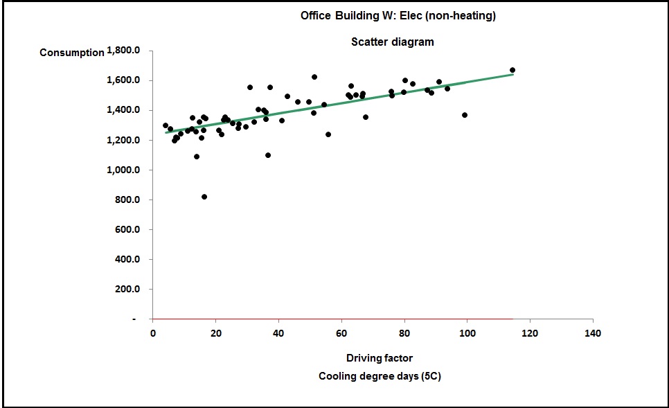
The gradient of this line is 3.5 kWh per (cooling) degree day. It is of similar order to the 6.1 kWh per degree day for heating, which is to be expected; the building’s heat loss and gain rates per degree difference are likely to be similar. As importantly, we now have an intercept on the vertical axis (a shade over 1,200 kWh per week) which represents the non-weather-related demand. Taking Figure 1 at face value we would have erroneously put the fixed consumption at around 1,500 kWh per week.
Also significant is the fact that Figure 4 was plotted against cooling degree days to a base of only 5°C. That was the only way to get a rational straight line and it means there is a finite amount of cooling going on at outside temperatures down to that value. I had been assured that cooling was only enabled “when the weather got hot”. But plotting demand against cooling degree days to, say, 15.5°C (a common default for summer-only use) gave the result shown in Figure 5:
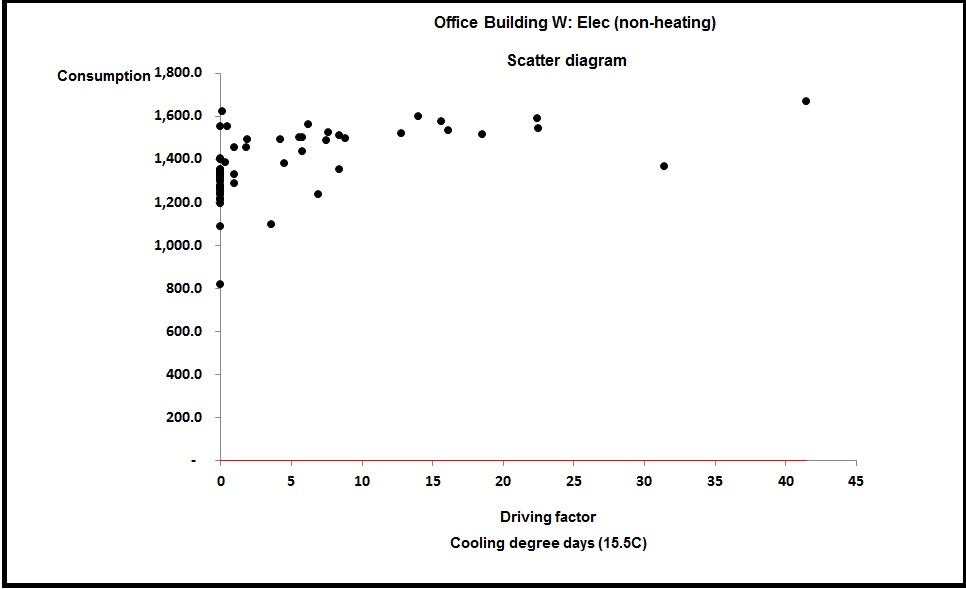
This is not as good a correlation as Figure 4 and my conclusion in this case was that when the outside temperature is between 5 and 12°C, this building is likely to have some rooms heating and some cooling.