Anyone familiar with the principles of monitoring and targeting (M&T) and measurement and verification (M&V) will recognise the overlap between the two. Both involve establishing the mathematical relationship between energy consumption and one or more independently-variable ‘driving factors’, of which one important example would be the weather expressed numerically as heating or cooling degree days.

One of my clients deals with a huge chain of retail stores with all-electric services. They are the subject of a rolling refit programme, during which the opportunity is taken to improve energy performance. Individually the savings, although a substantial percentage, are too small in absolute terms to warrant full-blown M&V. Nevertheless he wanted some kind of process to confirm that savings were being achieved and to estimate their value.

My associate Dan Curtis and I set up a pilot process dealing in the first instance with a sample of a hundred refitted stores. We used a basic M&T analysis toolkit capable of cusum analysis and regression modelling with two driving factors, plus an overspend league table (all in accordance with Carbon Trust Guide CTG008). Although historical half-hourly data are available we based our primary analysis on weekly intervals.

The process

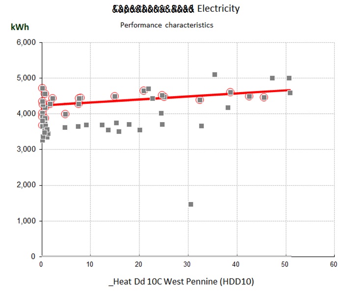
The scheme will work like this. After picking a particular dataset for investigation, the analyst will identify a run of weeks prior to the refit and use their data establish a degree-day-related formula for expected consumption. This becomes the baseline model (note that in line with best M&V practice we talk about a ‘baseline model’ and not a baseline quantity; we are interested in the constant and coefficients of the pre-refit formula). Here is an example of a store whose electricity consumption was weakly related to heating degree days prior to its refit:

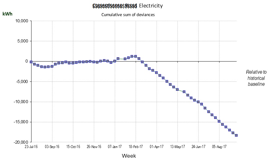
Cusum analysis using this baseline model yields a chart which starts horizontal but then turns downwards when the energy performance improves after the refit:

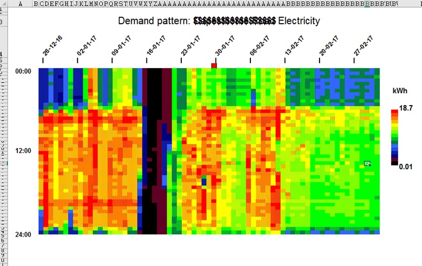
Thanks to the availability of half-hourly data, the M&T software can display a ‘heatmap’ chart showing half-hourly consumption before, during and after the refit. In this example it is interesting to note that savings did not kick in until two weeks after completion of the refit:

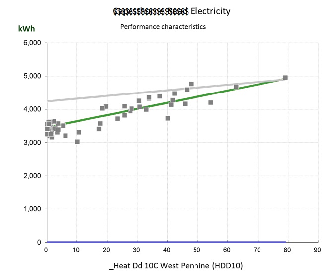
Once enough weeks have passed (as in the case under discussion) the analyst can carry out a fresh regression analysis to establish the new performance characteristic, and this becomes the target for every subsequent week. The diagram below shows the target (green) and baseline (grey) characteristics, at a future date when most of the pre-refit data points are no longer plotted:

A CTG008-compliant M&T scheme retains both the baseline and target models. This has several benefits:

• Annual savings can be projected fairly even if the pre- or post-refit periods are less than a year;
• The baseline model enables savings to be tracked objectively: each week’s ‘avoided energy consumption’ is the difference between actual consumption and what the baseline model yielded as an estimate (given the prevailing degree-day figures); and
• The target model provides a dynamic yardstick for ongoing weekly consumptions. If the energy-saving measures cease to work, actual consumption will exceed what the target model predicts (again given the prevailing degree-day figures). See final section below on routine monitoring.

I am covering advanced M&T methods in a workshop on 11 September in Birmingham

A legitimate approach?

Doing measurement and verification this way is a long way off the requirements in IPMVP. In the circumstances we are talking about – a continuous pipeline of refits managed by dozens of project teams – it would never be feasible to have M&V plans for every intervention,. Among the implications of this is that no account is taken (yet) of static factors. However, the deployment of heat-map visualisations means that certain kinds of change (for example altered opening hours) can be spotted easily, and others will be evident. I would expect that with the sheer volume of projects being monitored, my client will gradually build up a repertoire of common static-factor events and their typical impact. This makes the approach essentially a pragmatic one of judging by results after the event; the antithesis of IPMVP, but much better aligned to real-world operations.

Long-term routine monitoring

The planned methodology, particularly when it comes to dealing with erosion of savings performance, relies on being able to prioritise adverse incidents. Analysts should only be investigating in depth cases where something significant has gone wrong. Fortunately the M&T environment is perfect for this,  since ranked exception reporting is one of its key features. Every week, the analyst will run the Overspend League Table report which ranks any discrepancies in descending order of apparent weekly cost:

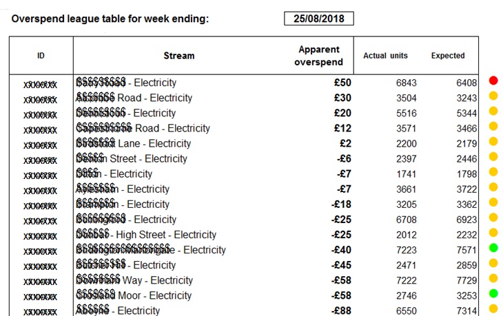
Any important issues are therefore at the top of page 1, and a significance flag is also provided: a yellow dot indicating variation within normal uncertainty bands, and a red dot indicating unusually high deviation. Remedial effort can then be efficiently targeted, and expected-consumption formulae retuned if necessary.