Background: conventional energy monitoring

In classic monitoring and targeting practice, consumption is logged at regular intervals along with relevant associated driving factors and a formula is derived which computes expected consumption from those factors. A common example would be expected fuel consumption for space heating, calculated from measured local degree-day values via a simple straight-line relationship whereby expected consumption equals a certain fixed amount per week plus so many kWh per degree-day. Using this simple mathematical model, weekly actual consumptions can then be judged against expected values to reveal divergence from efficient operation regardless of weather variations. The same principle applies in energy-intensive manufacturing, external lighting, air compressors, vehicles and any other situation where variation in consumption is driven by variation in one or more independently measurable factors. The expected-consumption models may be simple or complex.

Comparing actual and expected consumptions through time gives us valuable graphical views such as control charts and cusum charts. These of course rely on the data being sequential, i.e., in the correct chronological sequence, but they do not necessarily need the data to be consecutive. That is to say, it is permissible to have gaps, for instance to skip invalid or missing measurements.

The Brigadoon method

“Brigadoon” is a 1940s Broadway musical about a mythical Highland village that appears in the real world for only one day a year (although as far as its inhabitants are concerned time is continuous) and its plot concerns two tourists who happen upon this remote spot on the day that the village is there. The story came to mind some years ago when I was struggling to deal with energy monitoring of student residences. Weekly fuel consumption naturally dropped during vacations (or should do) and I realised I would need two different expected-consumption models, one for occupied weeks and another for unoccupied weeks using degree-days computed to a lower base temperature. One way to accommodate this was to have a single more complex model that took the term/vacation state into account. In the event I opted for splitting the data history into two: one for term weeks, and the other for vacation weeks. Each history thus had very long gaps in it, but there is no objection to closing up the gaps so that in effect the last week of each term is immediately followed by the first week of the next and likewise for vacations.

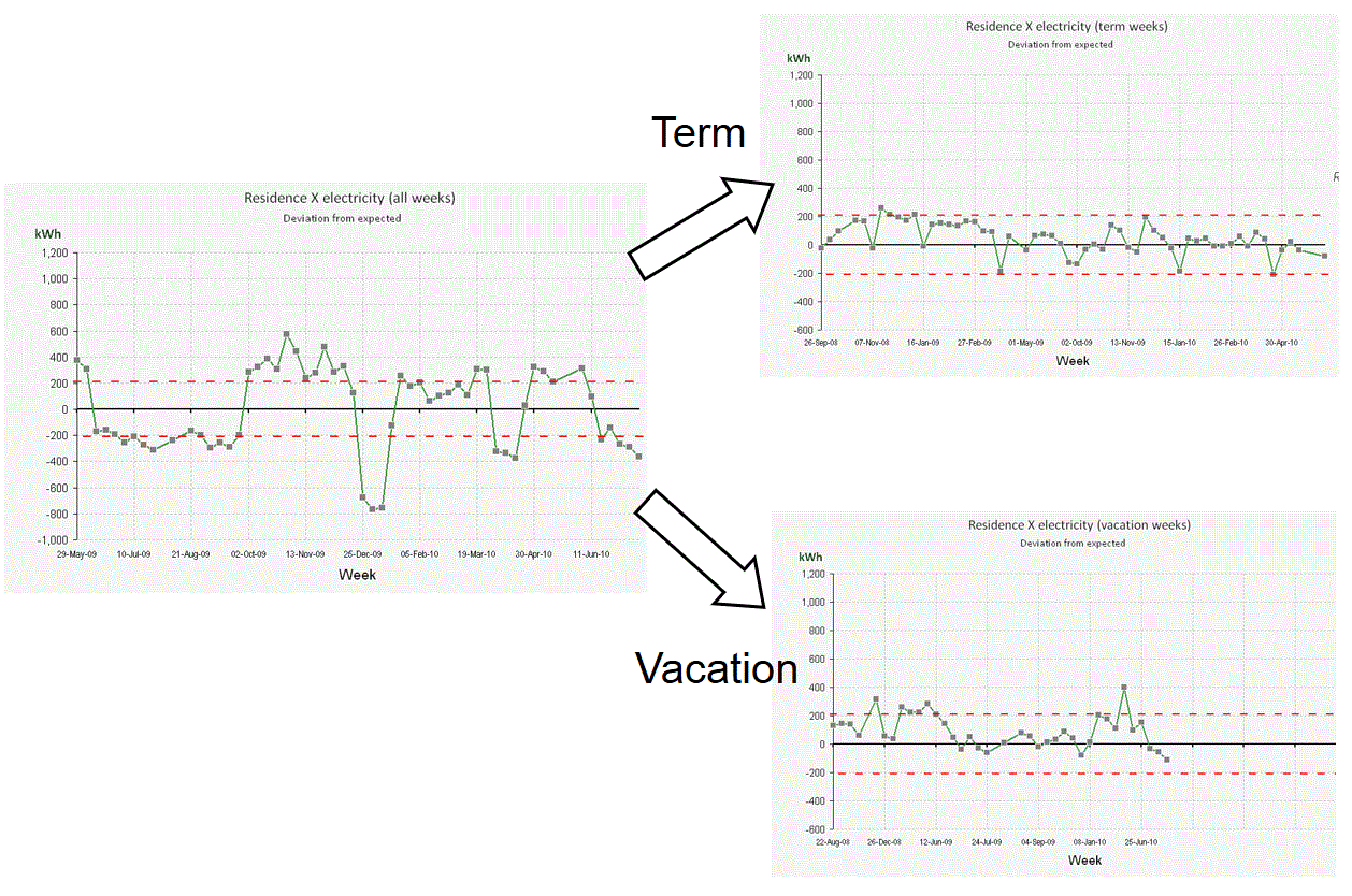
This strategy made the single building into two different ones. Somewhat like Brigadoon, the ‘vacant’ manifestation of the building for instance only comes into existence outside term time, but it appears to have a continuous history. The diagram below shows the control chart using a single degree-day model on the left, as per conventional practice, while on the right we see the separate control charts for the two virtual buildings, plotted with the same limits to show the reduction in modelling error.

Not just space heating

This principle can be used in many situations. I have used it very successfully on distillation columns in a chemical works to eliminate non-steady-state operation. I recommended it for a dairy processing plant with automatic meter reading where the night shift only does cleaning while the day shift does production: the meters can be read at shift change to give separate ‘active’ and ‘cleaning’ histories for every week. A friend recently asked me to look at data collected from a number of kilns with batch firing times extending over days, processing different products; here it will be possible to split the histories by firing programme: one history for programme 20, another for 13, and so on.