Suppose you want to analyse the relationship between consumption and its most significant driving factor, but you know that there is a secondary influence which will distort the result if you don’t take account of it. The easy way to approach this is to analyse historical data statistically using multiple regression, which will estimate the fixed consumption and give you the sensitivities to both variable driving factors.
Unfortunately, in a world where you cannot guarantee that the thing you are analysing has previously behaved in a consistent manner, this statistically-derived guess at the relationship could well be wrong. It will also be unreliable if, for example, the secondary driving factor does not vary very much.
We must bear in mind that statistical analysis has no insight into physical reality and can therefore generate implausible answers. Because of this, I always recommend using non-statistical methods of establishing how consumption responds to variation in a given driving factor. One way is to go back to first principles. Daylight-linked lighting demand provides an excellent example. If you have, say, 500 watts capacity of photocell-controlled lighting, you know for sure that it will use 0.5 kWh for each hour of darkness. Weekly and monthly hours of darkness (HD) can be obtained from standard tables and thus, for any given week or month, you can say how much electricity that lighting installation will use: it’s just 0.5 x HD. What we can do now is ‘net back’ our historical energy consumptions by deducting 0.5 x HD from the metered totals. This removes a calculated allowance for external lighting and the net consumption can then legitimately be analysed against the primary driving factor alone.
Netting-back can be used in other circumstances. On one occasion I was trying to model expected electricity consumption for cooling a computer data centre. Obviously cooling degree days are one driving factor here, but cooling demand would also be sensitive to the amount of electricity fed to the computers housed in the building (for every kWh consumed in the equipment racks, some fraction of a kWh is needed to provide the corresponding cooling). If the rack power were constant week by week, it would not be a problem, as the consequent cooling requirement would appear as part of the fixed electricity demand. On the other hand if it varied widely from week to week it would not be a problem either, because regression analysis would then have a fighting chance. The difficulty was that rack power did vary, but not very often and usually not by very much. The practical solution here was to assume a coefficient of performance for the chillers and to say that their demand would vary by 0.3 kWh per kWh of electricity delivered to equipment racks. Although this was more of an educated guess than an actual measurement, any error in the estimated coefficient was very much diluted in the overall expected-consumption model and on balance the model was more accurate than it would have been if the factor were ignored.
Want training on energy monitoring and targeting? Check the listings at http://vesma.com/training
A case history
I’ll conclude with a story where regression analysis was problematic and a netting-back approach had to be used.
The story concerns an all-electric building which at the outset I had not yet visited, but for which I had energy data. Since no heating fuel was involved, I started by analysing electricity consumption against heating degree days only, which yielded the result shown in Figure 1. Consumption is predominantly fixed:
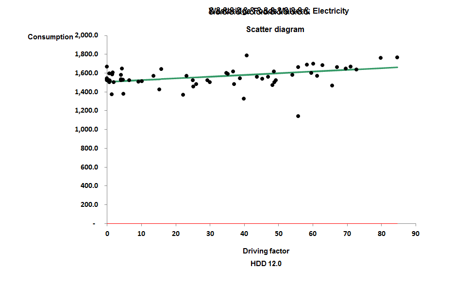
The gradient of the line, at 1.4 kWh/HDD, was troublingly low. Finding that the building had reversible heat pumps I concluded that I was looking at the combined overlapping effect of seasonal heating and cooling.
As there was good information on the thermal performance of the building I was able to estimate what the gradient of the line should have been in theory. It came out at 5.8 kWh/HDD. This enabled me to net back the historical totals to get figures for non-heating consumption, which, when analysed against cooling degree days, gave me Figure 2:
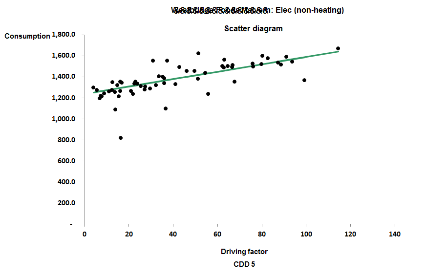
The gradient of the cooling relationship came out at 3.5 kWh/CDD.
Out of interest I also subjected the data to multiple regression analysis. This yielded an estimate of fixed consumption similar to the other methods but underestimated the coefficients of the two driving factors. It gave a heating degree-day coefficient of 3.6 kWh/HDD (compared with 5.8 based on the building’s physical characteristics) and a cooling coefficient of 1.8 kWh/CDD compared with the 3.5 derived above. It is always problematic when heating and cooling degree days both apply as driving factors, because they are not the completely independent variables that statistical theory demands.
Summary
‘Netting back’ is a useful strategy when consumption has two or more driving factors and you do not want to rely entirely on regression analysis. It is particularly useful when
- You have a good method of determining a coefficient from first principles, or empirically from a deliberate test;
- You have a known driving factor which varies only slightly or changes infrequently;
- You have driving factors that are not completely independent