All posts by Editor

Energy after Brexit

DATELINE 1 APRIL, 2019: Thinking about the laws that are likely to change post-EU, the most significant from an energy standpoint are the laws of science, meaning it is likely that:

  1. fuels will become susceptible to magnetism, enabling even more complete combustion than can be obtained through proper maintenance;
  2. the internal metallic layers in multi-foil insulation will be able to reflect heat back through the adjoining insulant and out through the surface foil;
  3. heating-water additives will enable radiators to heat up quicker but release heat more slowly;
  4. boiler anti-cycling devices that cut fuel consumption during periods of low load will do the same under medium and high load conditions which account for the majority of annual fuel consumption;
  5. insulating paints will be as effective as conventional insulation materials that are 4,000 times thicker;
  6. temperature sensors in freezers will respond more accurately and rapidly when encased in a cube of gel;
  7. putting solar panels in refrigeration circuits will enable even more heat to be pumped out with the same electrical input;
  8. ‘kinetic’ pavements will generate enough energy to power a display showing how many steps passing people have taken; and
  9. voltage-reduction devices will enable electrical equipment to perform the same work with lower energy input, and will themselves no longer incur standing power losses.

These insights are provided courtesy of Laboratoires Farage.

Uncertainty in savings estimates: a worked example

To prove that energy performance has improved, we calculate the energy performance indicator (EnPI) first for a baseline period and again during the subsequent period which we wish to evaluate. Let us represent the baseline EnPI value as P1 and the subsequent period’s value as P2

Most people would then say that as long as P2 is less than Pwe have proved the case. But there is uncertainty in both P1 and P2 and this will be translated into uncertainty in the estimate of their difference. We strictly need to show not only that the difference (P1 – P2) is positive, but that the difference exceeds the uncertainty in its calculation. Here’s how we can do that.

In the example which follows I will use a particular form of EnPI called the ‘Energy Performance Coefficient’ (EnPC), although any numerical indicator could be used. The EnPC is the ratio of actual to expected consumption. By definition this has a value of 1.00 over your baseline period, falling to lower values if energy-saving measures result in consumption less than otherwise expected. To avoid a long explanation of the statistics I’ll also draw on Appendix B of the International Performance Measurement and Verification Protocol (IPMVP, 2012 edition) which can be consulted for deeper explanations.

IPMVP recommends evaluation based on the Standard Error, SE, of (in this case) the EnPC. To calculate SE you first calculate the EnPC at regular intervals and measure the Standard Deviation (SD) of the results; then divide SD by the square root of the number of EnPI observations. In my sample data I use 2016 and 2017 as the baseline period, and calculate the EnPC month by month.

In my sample data the standard deviation of the EnPC during the baseline period was 0.04423 and there being 24 observations the baseline Standard Error was thus

SE1 = 0.04423 / √24 = 0.00903

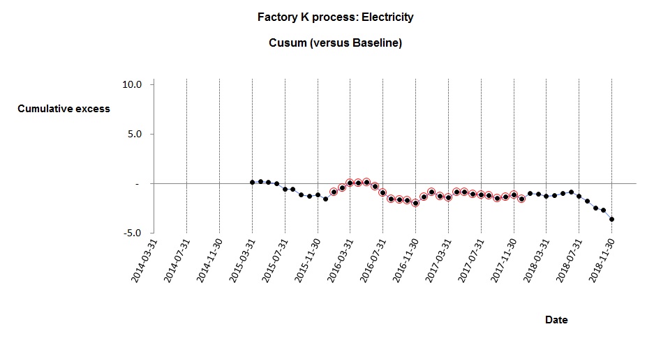
Here is the cusum analysis with the baseline observations highlighted:

The cusum analysis shows that performance continued unchanged after the baseline period but then in July 2018 it improved. We see that the final five months show apparent improvement; the mean EnPC after the change was 0.94, and these five observations had a Standard Deviation of 0.02402. Their Standard Error was therefore

SE2 = 0.02402 / √5 = 0.01074

SEdiff , the Standard Error of the difference (P1 – P2) is given by

SEdiff = √( SE12 + SE22 )

= √( 0.009032 + 0. 010742 )

= 0.01403

SE on its own does not express the true uncertainty. It must be multiplied by a safety factor t which will be smaller if we have more observations (or if we can accept lower confidence) and vice versa. This table is a subset of t values cited by IPMVP:

	     |     Confidence level     |
             |   90%  |   80%  |   50%  |
Observations |        |        |        |
      5      |  2.13  |  1.53  |  0.74  |
     10      |  1.83  |  1.38  |  0.70  |
     12      |  1.80  |  1.36  |  0.70  |
     24      |  1.71  |  1.32  |  0.69  |
     30      |  1.70  |  1.31  |  0.68  |

Let us suppose we want to be 90% confident that the true reduction in the EnPC lies within a certain range. We therefore need to pick a t-value from the “90%” column of the table above. But do we pick the value corresponding to 24 observations (the baseline case) or 5 (the post-improvement period)? To be conservative—as required by IPMVP—we take the lower number, meaning we must in this case use a t value of 2.13.

Now in the general case ∆P, the EnPC reduction, is given by

∆P = (P1 – P2) ± t.SEdiff

Which, substituting the values from our example, would yield

∆P = (1.00 – 0.94) ± (2.13 x 0.01403)

∆P = 0.06 ± 0.03

The lowest probable value of the improvement ∆P is thus (0.06 – 0.03) = 0.03 . It may in reality be less, but the chances of that are only 1 in 20 because we are 90% confident that it falls within the stated range and by implication 5% confident that it is above the upper limit.

Footnote: example data

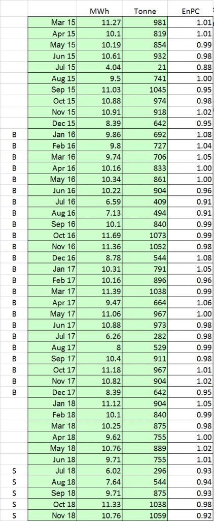
The analysis is based on real data (preview below). These are from an anonymous source and  multiplied by a secret factor to disguise their true values. Anybody wishing to verify the analysis can download the anonymous data as a spreadsheet here.

Note: to compute the baseline EnPC

  1. do a regression of MWh against tonnes using the months labelled ‘B’
  2. create a column of ‘expected’ consumptions by substituting tonnage values in the regression formula 
  3. divide each actual MWh figure by the corresponding expected value

Product awards: handle with care

This article may upset some of my friends in at energy publications and associations, but we have a problem which people need to be aware of. It is that we can no longer trust awards for energy-saving products as indicators of merit.

I get asked for advice about dubious products by my newsletter readers and often they’ll say “I smell a rat but it has an award from [insert name of prestigious body]“. How can something bogus get an award that it does not deserve? To  answer that you have to understand how award schemes work. In particular you need to appreciate that their promoters are driven by profit. The commercial imperative is simple: get as many bums on expensive seats as possible at a gala-dinner awards ceremony. To do that, they need to have a lot of short-listed candidates, because those are the people who will pay on the off-chance that they get to pose as a winner with the celebrity host. Having a big shortlist means putting an awful lot of entries in front of the judging panel (44 for one  panel I sat on). But these judges are unpaid, and as volunteers they simply cannot spare enough time to scrutinise entries thoroughly, even though some do take it seriously and try to be diligent. They aren’t helped by the fact that candidates often submit little more than rehashed sales blurbs full of unsubstantiated claims — a short-cut which promoters condone in the interests of maximising the number of bums on seats.

Some judges, moreover, will have been selected more for their celebrity than their knowledge (celebrity judges equals more bums on seats), and will lack the ability to spot snake-oil propositions or even to understand counter-arguments from more knowledgeable fellow-judges. The majority of any panel will be easily swayed by the plausible nonsense in the entries, will not question the credibility of testimonials, and will naively assume that no competition entrant could possibly have criminal intent.

It is asymmetric warfare. The snake-oil peddler just needs to keep plugging away with award entries because the spurious credibility that they get from their first award is too valuable to forego. Once they have landed one award, they are effectively immunised against rejection by judges for other awards and probably even have their chances boosted.

I don’t want to tar all awards with the same brush: in an honest world they would all work to everyone’s benefit, and no promoter is knowingly complicit in the occasional fraud that slips through the net. But sadly a few bad apples have devalued energy awards and my advice would be this. If you have doubts about a product,  seeing the phrase ‘award-winning’ should put you on alert.

“Science-based targets”: sounds good, means very little

WHEN I FIRST heard the term science-based target (SBT) bandied around in the public arena I thought “oh good – they are advocating a rational approach to energy management”. I thought they were promoting the idea that I always push, which is to compare your actual energy consumption against an expected quantity calculated, on a scientific basis, from the prevailing conditions of weather, production activity, or whatever other measurable factors drive variation in consumption.

How wrong I was. Firstly, SBTs are targets for emissions, not energy consumption;  and secondly a target is defined as ‘science-based’ if, to quote the Carbon Trust, “it is in line with the level of decarbonisation required to keep the global temperature increase below 2°C compared to pre-industrial temperatures”. I have three problems with all of this.

Firstly I have a problem with climate change. I believe it is real, of course; and I am sure that human activity, fuel use in particular, is the major cause. What I don’t agree with is using it as a motivator or to define goals. It is too remote, too big, and too abstract to be relevant to the individual enterprise. And it is too contentious. To mention climate change is to invite debate: to debate is to delay.

Secondly, global targets cannot be transcribed directly into local ones. If your global target is a reduction of x% and you set x% as the target for every user, you will fail because some people will be unable or unwilling to achieve a cut of x% while those who do achieve x% will stop when they have done so. In short there will be too few over-achievers to compensate for the laggards.

Finally I object to the focus on decarbonisation. Not that decarbonisation itself is valueless; quite the opposite. It is the risk that people prioritise decarbonisation of supply, rather than reduction of demand. If you decarbonise the supply to a wasteful operation, you have denied low-carbon energy to somebody somewhere who needed it for a useful purpose. We should always put energy saving first, and that is where effective monitoring and targeting, including rational comparisons of actual and expected consumption, has an essential part to play.

Bulk measurement and verification

Anyone familiar with the principles of monitoring and targeting (M&T) and measurement and verification (M&V) will recognise the overlap between the two. Both involve establishing the mathematical relationship between energy consumption and one or more independently-variable ‘driving factors’, of which one important example would be the weather expressed numerically as heating or cooling degree days.

One of my clients deals with a huge chain of retail stores with all-electric services. They are the subject of a rolling refit programme, during which the opportunity is taken to improve energy performance. Individually the savings, although a substantial percentage, are too small in absolute terms to warrant full-blown M&V. Nevertheless he wanted some kind of process to confirm that savings were being achieved and to estimate their value.

My associate Dan Curtis and I set up a pilot process dealing in the first instance with a sample of a hundred refitted stores. We used a basic M&T analysis toolkit capable of cusum analysis and regression modelling with two driving factors, plus an overspend league table (all in accordance with Carbon Trust Guide CTG008). Although historical half-hourly data are available we based our primary analysis on weekly intervals.

The process

The scheme will work like this. After picking a particular dataset for investigation, the analyst will identify a run of weeks prior to the refit and use their data establish a degree-day-related formula for expected consumption. This becomes the baseline model (note that in line with best M&V practice we talk about a ‘baseline model’ and not a baseline quantity; we are interested in the constant and coefficients of the pre-refit formula). Here is an example of a store whose electricity consumption was weakly related to heating degree days prior to its refit:

Cusum analysis using this baseline model yields a chart which starts horizontal but then turns downwards when the energy performance improves after the refit:

Thanks to the availability of half-hourly data, the M&T software can display a ‘heatmap’ chart showing half-hourly consumption before, during and after the refit. In this example it is interesting to note that savings did not kick in until two weeks after completion of the refit:

Once enough weeks have passed (as in the case under discussion) the analyst can carry out a fresh regression analysis to establish the new performance characteristic, and this becomes the target for every subsequent week. The diagram below shows the target (green) and baseline (grey) characteristics, at a future date when most of the pre-refit data points are no longer plotted:

A CTG008-compliant M&T scheme retains both the baseline and target models. This has several benefits:

  • Annual savings can be projected fairly even if the pre- or post-refit periods are less than a year;
  • The baseline model enables savings to be tracked objectively: each week’s ‘avoided energy consumption’ is the difference between actual consumption and what the baseline model yielded as an estimate (given the prevailing degree-day figures); and
  • The target model provides a dynamic yardstick for ongoing weekly consumptions. If the energy-saving measures cease to work, actual consumption will exceed what the target model predicts (again given the prevailing degree-day figures). See final section below on routine monitoring.

I am covering advanced M&T methods in a workshop on 11 September in Birmingham

A legitimate approach?

Doing measurement and verification this way is a long way off the requirements in IPMVP. In the circumstances we are talking about – a continuous pipeline of refits managed by dozens of project teams – it would never be feasible to have M&V plans for every intervention,. Among the implications of this is that no account is taken (yet) of static factors. However, the deployment of heat-map visualisations means that certain kinds of change (for example altered opening hours) can be spotted easily, and others will be evident. I would expect that with the sheer volume of projects being monitored, my client will gradually build up a repertoire of common static-factor events and their typical impact. This makes the approach essentially a pragmatic one of judging by results after the event; the antithesis of IPMVP, but much better aligned to real-world operations.

Long-term routine monitoring

The planned methodology, particularly when it comes to dealing with erosion of savings performance, relies on being able to prioritise adverse incidents. Analysts should only be investigating in depth cases where something significant has gone wrong. Fortunately the M&T environment is perfect for this,  since ranked exception reporting is one of its key features. Every week, the analyst will run the Overspend League Table report which ranks any discrepancies in descending order of apparent weekly cost:

Any important issues are therefore at the top of page 1, and a significance flag is also provided: a yellow dot indicating variation within normal uncertainty bands, and a red dot indicating unusually high deviation. Remedial effort can then be efficiently targeted, and expected-consumption formulae retuned if necessary.

Monitoring external lighting

The diagram below shows the relationship, over the past year, between weekly electricity consumption and the number of hours of darkness per week for a surface car park. It is among the most consistent cases I have ever seen:

Figure 1: relationship between kWh and hours of darkness


There is a single outlier (caused by meter error).

Although both low daylight availability and cold weather occur in the winter, heating degree days cannot be used as the driving factor for daylight-linked loads.  Plotting the same consumption data against heating degree days gives a very poor correlation:

Figure 2: relationship between kWh and heating degree days

There are two reasons for the poor correlation. One is the erratic nature of the weather (compared with very regular variations in daylight availability) and the other is the phase difference of several weeks between the shortest days and the coldest weather. If we co-plot the data from Figure 2 as a time-series chart we see this illustrated perfectly. In Figure 3 the dots represent actual electricity consumption and the green trace shows what consumption was predicted by the best-fit relationship with heating degree days:

Figure 3: actual kWh compared with a weather-linked model of expected consumption

Compare Figure 3 with the daylight-linked model:

Figure 4: actual and expected kWh co-plotted using daylight-linked model

One significant finding (echoed in numerous other cases) is that it is not necessary to measure actual hours of darkness: standard weekly figures work perfectly well. It is evident that occasional overcast and variable cloud cover do not introduce perceptible levels of error. Moreover, figures for UK appear to work acceptably at other latitudes: the case examined here is in northern Spain (41°N) but used my standard darkness-hour table for 52°N.

You can download my standard weekly and monthly hours-of-darkness tables here.

This article is promoting my advanced energy monitoring and targeting workshop in Birmingham on 11 September


Project sketch: vetting product offers

My client in this case is an international hotel brand. Individual hotels get approached by people selling questionable energy-saving products and rarely if ever have enough knowledge to defend themselves against bogus and exaggerated offers.

The company has established a core group of engineers and sustainability staff to carry out centralised vetting. My job is to provide technical advice during the initial filtering phase and to join a twice-yearly meeting to interview suppliers who are being taken further.

Project sketch: user requirement specification

Our client, a university, has a long-established metering system based on proprietary hardware with associated software for managing and interrogating the meters and storing their output for use, among other things, in a monitoring and targeting scheme. They have two major stakeholders, one predominantly interested in monitoring and managing power quality and availability, and the other in billing the various user departments. The existing scheme suffers from certain limitations and the client is considering migrating to a new data-collection provider. Continue reading Project sketch: user requirement specification