To prove that energy performance has improved, we calculate the energy performance indicator (EnPI) first for a baseline period and again during the subsequent period which we wish to evaluate. Let us represent the baseline EnPI value as P1 and the subsequent period’s value as P2
Most people would then say that as long as P2 is less than P1 we have proved the case. But there is uncertainty in both P1 and P2 and this will be translated into uncertainty in the estimate of their difference. We strictly need to show not only that the difference (P1 – P2) is positive, but that the difference exceeds the uncertainty in its calculation. Here’s how we can do that.
In the example which follows I will use a particular form of EnPI called the ‘Energy Performance Coefficient’ (EnPC), although any numerical indicator could be used. The EnPC is the ratio of actual to expected consumption. By definition this has a value of 1.00 over your baseline period, falling to lower values if energy-saving measures result in consumption less than otherwise expected. To avoid a long explanation of the statistics I’ll also draw on Appendix B of the International Performance Measurement and Verification Protocol (IPMVP, 2012 edition) which can be consulted for deeper explanations.
IPMVP recommends evaluation based on the Standard Error, SE, of (in this case) the EnPC. To calculate SE you first calculate the EnPC at regular intervals and measure the Standard Deviation (SD) of the results; then divide SD by the square root of the number of EnPI observations. In my sample data I use 2016 and 2017 as the baseline period, and calculate the EnPC month by month.
In my sample data the standard deviation of the EnPC during the baseline period was 0.04423 and there being 24 observations the baseline Standard Error was thus
SE1 = 0.04423 / √24 = 0.00903
Here is the cusum analysis with the baseline observations highlighted: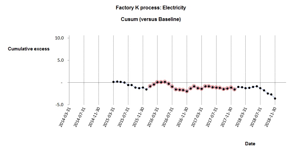
The cusum analysis shows that performance continued unchanged after the baseline period but then in July 2018 it improved. We see that the final five months show apparent improvement; the mean EnPC after the change was 0.94, and these five observations had a Standard Deviation of 0.02402. Their Standard Error was therefore
SE2 = 0.02402 / √5 = 0.01074
SEdiff , the Standard Error of the difference (P1 – P2) is given by
SEdiff = √( SE12 + SE22 )
= √( 0.009032 + 0. 010742 )
= 0.01403
SE on its own does not express the true uncertainty. It must be multiplied by a safety factor t which will be smaller if we have more observations (or if we can accept lower confidence) and vice versa. This table is a subset of t values cited by IPMVP:
	     |     Confidence level     |
             |   90%  |   80%  |   50%  |
Observations |        |        |        |
      5      |  2.13  |  1.53  |  0.74  |
     10      |  1.83  |  1.38  |  0.70  |
     12      |  1.80  |  1.36  |  0.70  |
     24      |  1.71  |  1.32  |  0.69  |
     30      |  1.70  |  1.31  |  0.68  |
Let us suppose we want to be 90% confident that the true reduction in the EnPC lies within a certain range. We therefore need to pick a t-value from the “90%” column of the table above. But do we pick the value corresponding to 24 observations (the baseline case) or 5 (the post-improvement period)? To be conservative—as required by IPMVP—we take the lower number, meaning we must in this case use a t value of 2.13.
Now in the general case ∆P, the EnPC reduction, is given by
∆P = (P1 – P2) ± t.SEdiff
Which, substituting the values from our example, would yield
∆P = (1.00 – 0.94) ± (2.13 x 0.01403)
∆P = 0.06 ± 0.03
The lowest probable value of the improvement ∆P is thus (0.06 – 0.03) = 0.03 . It may in reality be less, but the chances of that are only 1 in 20 because we are 90% confident that it falls within the stated range and by implication 5% confident that it is above the upper limit.
Footnote: example data
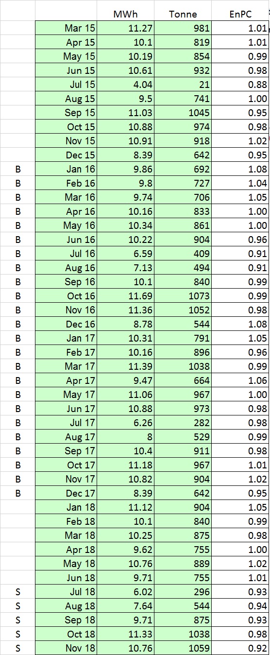
The analysis is based on real data (preview below). These are from an anonymous source and multiplied by a secret factor to disguise their true values. Anybody wishing to verify the analysis can download the anonymous data as a spreadsheet here.
Note: to compute the baseline EnPC
- do a regression of MWh against tonnes using the months labelled ‘B’
- create a column of ‘expected’ consumptions by substituting tonnage values in the regression formula
- divide each actual MWh figure by the corresponding expected value