This case history shows how fine-grained energy measurements enabled savings to be verified in the face of assorted practical problems.

THE STORY concerns a large air-conditioned establishment in the middle east which had been fitted with adiabatic cooling sprays on its central chillers. It is one of a number belonging to an international chain and my purpose was to establish whether similar technology should be contemplated elsewhere in the chain.

I had originally been commissioned to give a second opinion on the savings claims made by the equipment supplier. Although the claims were quite plausible, they lacked some credibility because they were based on an extremely short evaluation. So in an initial effort at  independent checking I obtained several years’ worth of monthly consumption data at the whole-site level and analysed it against local cooling degree days. The results were ambiguous because there appeared to be some unrelated phenomenon at play which resulted in the site toggling on a seasonal cycle between two performance characteristics, one significantly worse than the other, with an impact sufficient to mask the beneficial effect of the energy conservation measure (ECM).

Without reliable evidence I declined to verify the supplier’s assessment, and recommended a deliberate test using a ‘retrofit isolation’ approach based on three existing electricity submeters (one per chiller) and a new heat meter in the common chilled-water circuit. Because nobody wanted to pay for a proper heat meter, a clamp-on ultrasonic flow element was specified. At this point the pandemic struck.

Because we had data-logged metering, and because the adiabatic cooling system sounded as if it would lend itself to being turned on and off, the measurement and verification plan was based on day-on, day-off testing. I had proposed a ten-week testing campaign which would give us 35 observations in each state. The plan called for two regression models to be developed: one for the ECM ‘on’ days and the other for the ‘off’ days. Extrapolation from the regression formulae would indicate a percentage difference and variance within each would confirm how much uncertainty there was.

Then came the collision with reality. The ECM supplier said disabling it wasn’t as simple as turning the cooling sprays off; he insisted that the mesh screens which were part of the installation should come off as well and be reinstated when the spray was re-enabled. This was a quite reasonable stance because it gave a more valid comparison, but unfortunately he couldn’t afford to send a man to site every day to do what was necessary. Meanwhile the establishment’s manager had got wind of the project and put pressure on the site engineer not to disable the ECM, which he was convinced was saving him a lot of money which (thanks to lockdown) the business could not afford to lose. He also had a point. Luckily we agreed a compromise: in exchange for them coming down to a three-day on-off cycle, I promised to monitor things closely and terminate the test as soon as conclusive results emerged.

Needless to say, the ultrasonic meter let us down. The technician responsible for downloading its data reported that some of its hourly totals looked suspiciously high, and he proposed filtering them out. But I feared that he might not be able to capture all the rogue points. Some of them might only be slightly wrong, but wrong nonetheless. When we drilled down we discovered that the raw data were stored at one-minute intervals, with the measurement fault manifesting itself as gross errors confined to occasional one-minute records. You can see this from this figure, which spans several months but plots every single one-minute record:

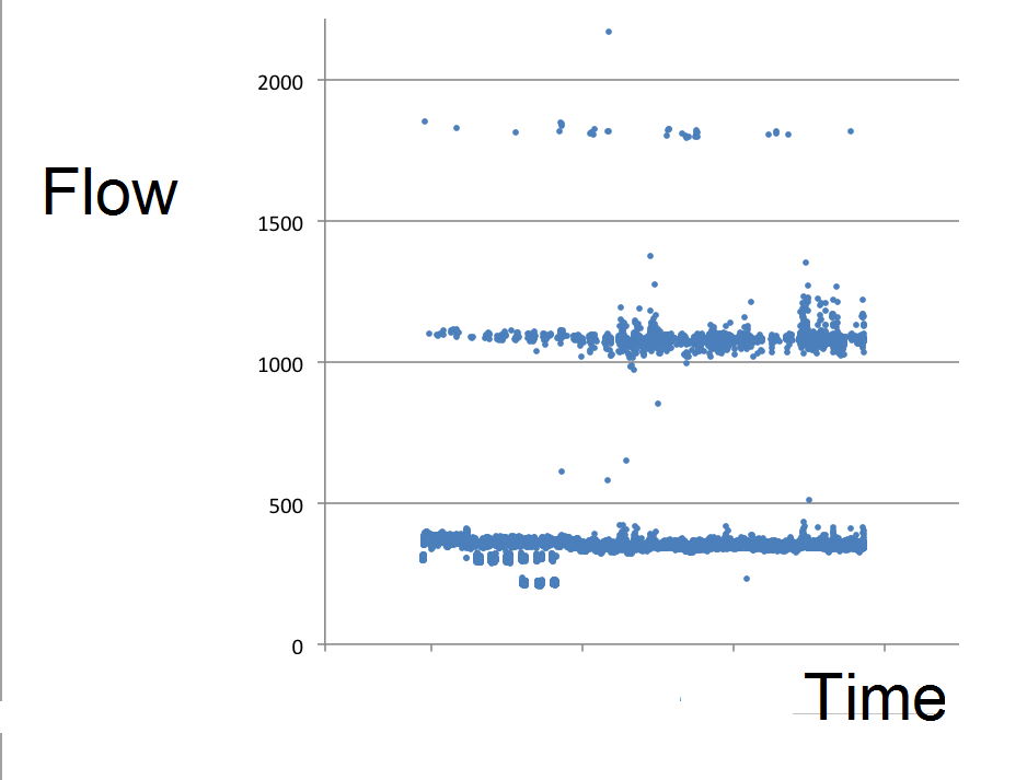
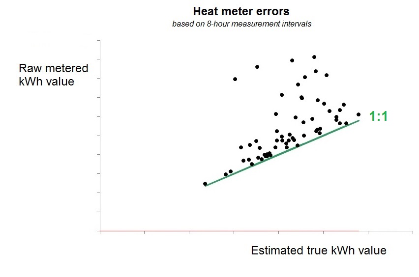
Valid readings at the one-minute interval clearly fell below a threshold of about 450 m3/hr, and abnormal readings were (a) very clear and (b) sparsely distributed through time, so my colleague Daniel Curtis was able to pushed the records through a sieve, take out the lumps and thereby cleanse the data (and that included reinstating hourly values which the meter software had censored because they appeared to be too low). We were helped in this by the flow normally being relatively constant, so that simple interpolation was an accurate gap-filling strategy. When we compared reported flow measurements with corrected values at eight-hour intervals we saw that in reality almost every reported value had been wrong:

Analysis then proceeded using cleaned-up eight-hour interval data, but we were still not out of the woods. From the individual chillers’ electricity meters we could see that the site operations team were changing the chiller sequence from time to time. Fortunately their manager agreed that barring emergencies they could leave the same chillers in service, with the same one in the lead, until the test finished. They also agreed not to change the chilled-water set point temperature, which we discovered they were in the habit of tweaking. Of course in a textbook measurement and verification exercise these static factors would have emerged during planning but this project was being conducted in a hurry on a shoestring and managed remotely. That wasn’t the end of it: later in the test we would have interruptions because the chiller maintenance firm was scheduled to clean the condenser coils. More on that later.

Nor were those the only complications. A few weeks after we started testing in anger in June, the plant did one of its random, unexplained and unexpected changes in energy performance. In Figure 3 you can see the deviation from predicted consumption for intervals when the ECM was active:

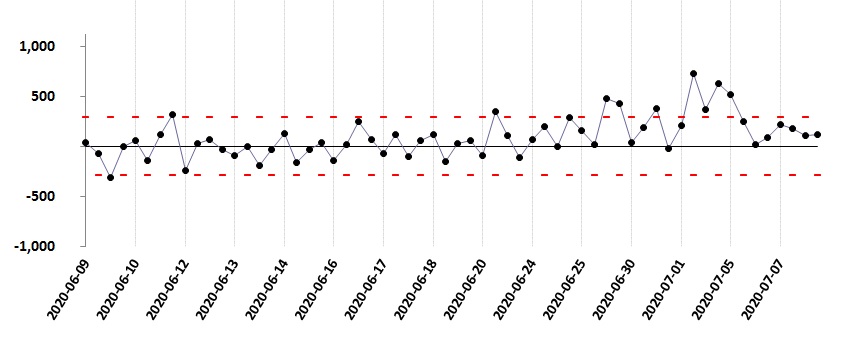
The chillers change their behaviour about two-thirds of the way through this history. If we look at the regression model for the ‘ECM on’ condition we can see the unexplained shift very clearly:

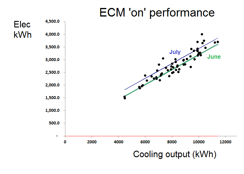
So we ended up, in effect, with two tests: one for June and one for July. Looking now at the comparison between ‘on’ and ‘off’ performance in July alone we saw a clear difference:

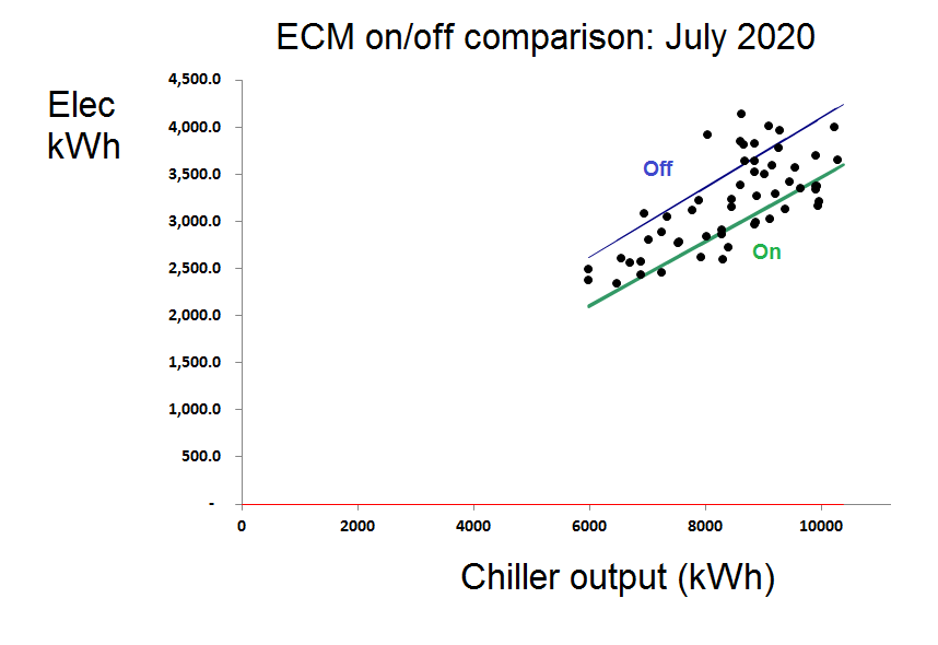
A similar picture was obtained from observations made in June and the conclusions were that savings of 16.1% and 17.5% were attributable to the ECM in June and July respectively. However, as a further bonus we observed:

• The chiller installation’s performance spontaneously deteriorated by 8% at the end of June, echoing behaviour first witnessed in 2019. Identifying the cause will probably save money quite easily; and
• Cleaning the condenser coils made no difference to performance. They were probably clean and it was a waste of money, so I suggested not cleaning them until condenser temperatures started to rise.

What lessons would I draw from this episode? That the verifier needs to be vigilant, sceptical, and cautious but flexible. In fact flexibility is needed on all sides, and that is best served by developing trust; trust in this case was built up through openness and continuous communication.